Create Data Validation List from Excel Table as Source

A common complaint of many Excel users is that they can’t directly use Excel table’s structured references in data validation to create drop-down lists.

If you try, Excel would give you an ugly pop-up and refuse to play along.

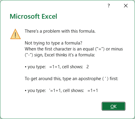
But what if you still want to (somehow) use Excel table as the source in data validation.

There is a work around – actually three workarounds.

In this article, I will show you how to use Excel Table as a source in data validation and how to create a drop down using it.

Using Excel Table as Source in Data Validation

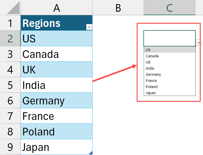
Below I have an Excel table (named ‘Data’), and I want to create a drop-down list that shows the list of all the countries in the Regions column.

Normally, I can refer to these country names by using a structured reference as shown below:

=Data[Regions]

where Data in the name of the table and Regions is the name of the column I am referring to.

But for some reason, Excel won’t allow me to use this structured reference in Data Validation.

So let’s see three ways to trick Excel and still use Excel Table structured reference in data validation.

Method 1: Using the INDIRECT Function

A quick and easy way to use Excel table in data validation is to put the structured reference within the INDRECT function

Here’s how you do it:

1. Select a cell where you want the drop-down
2. Go to the Data tab and click on the Data Validation icon

3. Select “List” from the Allow dropdown
4. In the Source field, enter:

=INDIRECT("Data[Regions]")

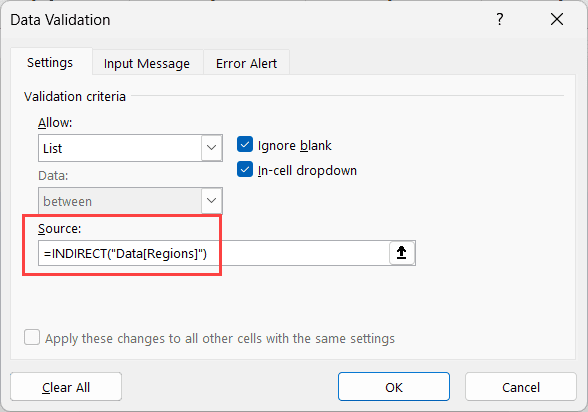
5. Click OK

This will give you functioning drop down list in the cell you selected in step 1

When you use INDIRECT function, instead of referring to the text “Data[Regions]”, it refers to what this name actually points to, which is your list of countries in the Region column.

And the best part? This is dynamic!

If you add or remove regions from your table, the drop-down list automatically updates.

This method also works across different sheets. So if your table is in one sheet and you want the drop-down in another sheet, no problem!

If you change the name of the table or the name of the column this method would break as the INDIRECT function would not know what to refer to. In case there is a possibility that you might change the name of the table or column it’s better to use the second method that uses Named Ranges

Method 2: Creating a Named Range with Structured Reference

This is the most reliable method to use Excel table in data validation.

In this method we first create a named range that would hold the reference to the table and then use this name range within the data validation dialog box.

Here’s is how it works:

1. Go to the Formulas tab and click on Define Name

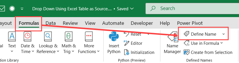
2. In the New Name dialog box, give your named range a name – let’s call it “RegionDD”
3. In the Refers to field, just use the structured reference: =Data[Regions]

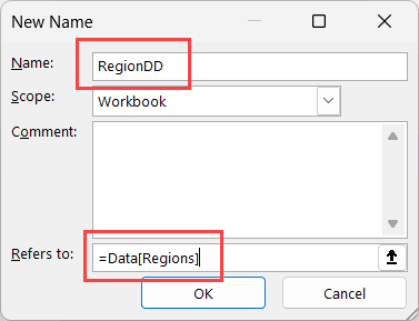
4. Click OK

The above steps have created a Named Range that we can now use in data validation using the below steps:

1. Go to the Data tab and click on the data validation icon
2. Select List from the Allow dropdown
3. In the Source field, enter: =RegionDD

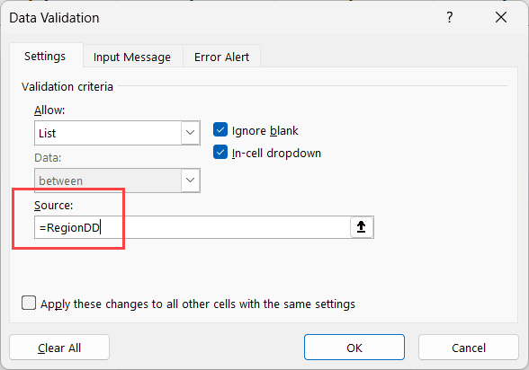
4. Click OK

This will give you a functioning drop down list that use Excel table column as the source.

Again, this method is dynamic. If you add anything to your regions list, the drop-down automatically expands. If you remove regions, the drop-down updates accordingly.

And even if you change the name of the table or the column this method would continue to work without any issues

Method 3: Direct Selection (Same Sheet Only)

And here’s a third workaround, which probably the easiest, but it has one limitation – this would only work if your Excel Table and the drop down are in the same worksheet.

Here is how this works:

1. Go to the Data tab and click on Data Validation icon
2. Select List from the Allow dropdown
3. Click in the Source field and simply select the cells in your table column

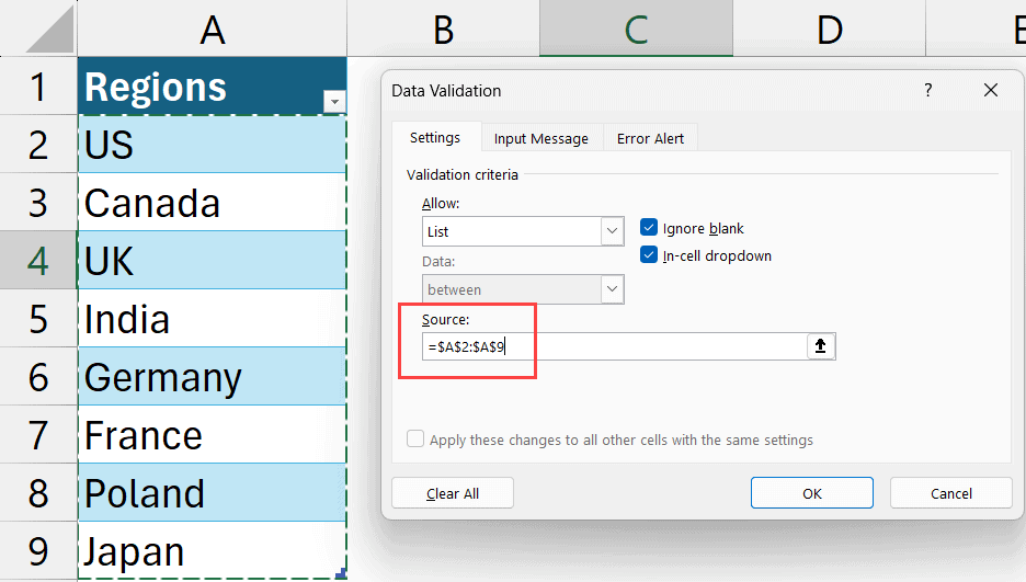
4. Click OK

This creates your drop-down list and it will automatically expand if you add new regions to your table.

But there is a limitation as I mentioned?

This only works if the Excel table and the drop-down list are in the same sheet. If they’re on different sheets, then this method won’t work as expected.

So there you have it – three ways to use table structured references in data validation drop-down lists.

I hope you found this useful! If you’re liking these Excel tips, make sure to keep an eye out for more tutorials like this one. Happy Excelling, and have a nice day!

Other Excel articles you may also like:

• Dependent Drop Down List in Excel
• Make a Yes/No Drop-Down in Excel
• Make Multiple Selections in a Drop Down List
• Show Symbols in Drop Down Lists
• Enable Conditional Data Entry using Data Validation