How to Make a Yes/No Drop-Down in Excel? (Easy Ways)

If you want to fill a column with Yes or No answers, typing them by hand gets slow, and someone will eventually make a mistake and type “yes ” or “Y”.

A Yes/No drop-down list fixes this. You simply pick Yes or No from the list, so there’s no room for misspelled words.

In this tutorial, I will show you two simple ways to create a Yes/No drop-down list in Excel. I’ll also show you how to color the answers and count them.

Create a Yes/No Drop-Down List by Typing the Values

The easiest way to create a Yes/No drop-down list is to type the values you want in the drop-down directly in the data validation dialog box.

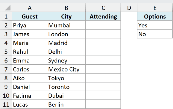
Below I have a list of guests for a team offsite in columns A and B. I want a Yes/No drop-down in column C so I can mark whether each person is attending.

Below are the steps to do this:

1. Select the cells where you want the drop-down (C2:C11 in this example).

2. Click the Data tab.

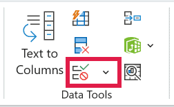
3. In the Data Tools group, click the Data Validation icon.

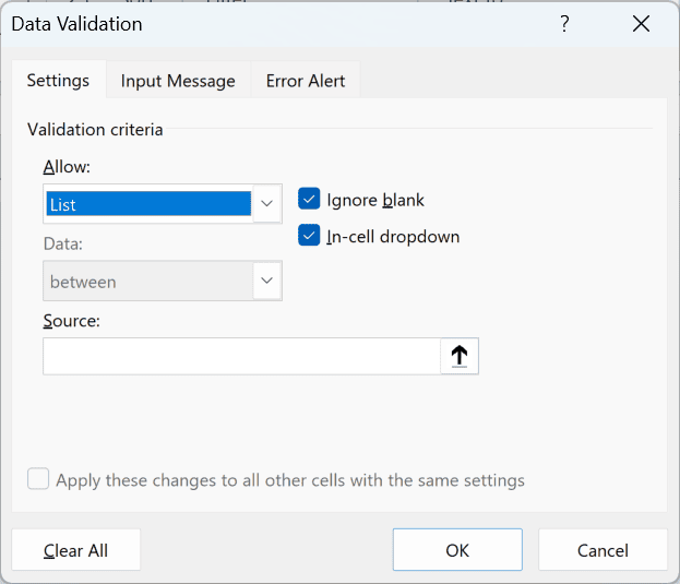
4. In the Data Validation dialog box, in the Settings tab, click the Allow drop-down and select List.

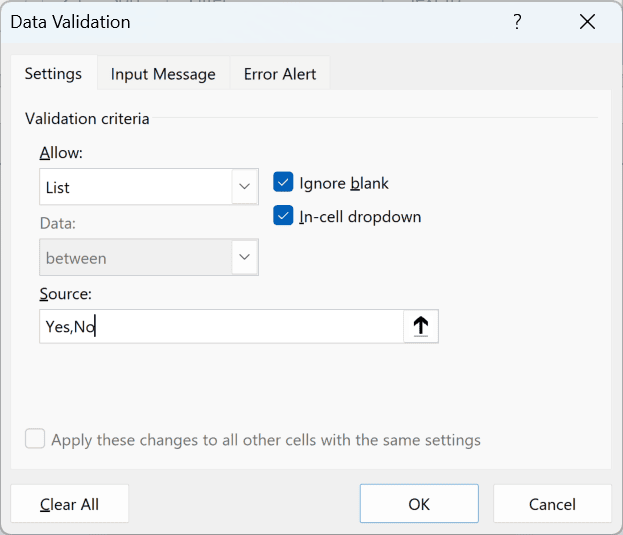
5. In the Source field, type Yes,No

6. Click OK.

Pro Tip: You can also open the Data Validation dialog box with the Windows keyboard shortcut ALT + A + V + V (select the cells first, then press these keys one after the other).

The above steps create a Yes/No drop-down in the selected cells. You’ll see a small drop-down arrow when you select any of these cells.

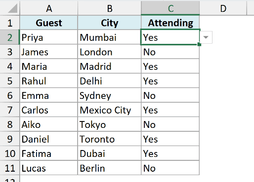
To pick a value, click the arrow and then select Yes or No.

You can also use the keyboard shortcut ALT + Down Arrow to open the drop-down (hold the ALT key and then press the down arrow key).

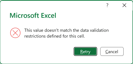
Once the drop-down is in a cell, you won’t be able to enter anything other than Yes or No. If you try, Excel shows an error box like the one below.

Important: If your Windows regional settings use a semicolon as the list separator (common in Europe), type Yes;No instead.

In this method, the drop-down values are hard-coded. To change the options later, you’ll have to go back to the Data Validation dialog box and make the changes there.

If you’d rather have a tick box than Yes/No text, use the new in-cell checkboxes in Microsoft 365 instead. They store TRUE or FALSE rather than Yes or No.

Create a Yes/No Drop-Down List Using a Cell Range

In the above method, we typed the Yes/No values into the Data Validation dialog box.

Another way is to enter the values in cells, and then use those cells as the source for the drop-down.

The benefit is that the drop-down becomes dynamic. If you change the values in those cells, the drop-down options change automatically.

Below I have the same guest list, and I want the Yes/No drop-down in column C. I also have Yes and No entered in cells E2 and E3.

Here are the steps to create a drop-down list using the values from these cells:

1. Select the cells where you want the drop-down (C2:C11).

2. Click the Data tab, and then click the Data Validation icon (it’s in the Data Tools group).

3. In the Settings tab, click the Allow drop-down and select List.

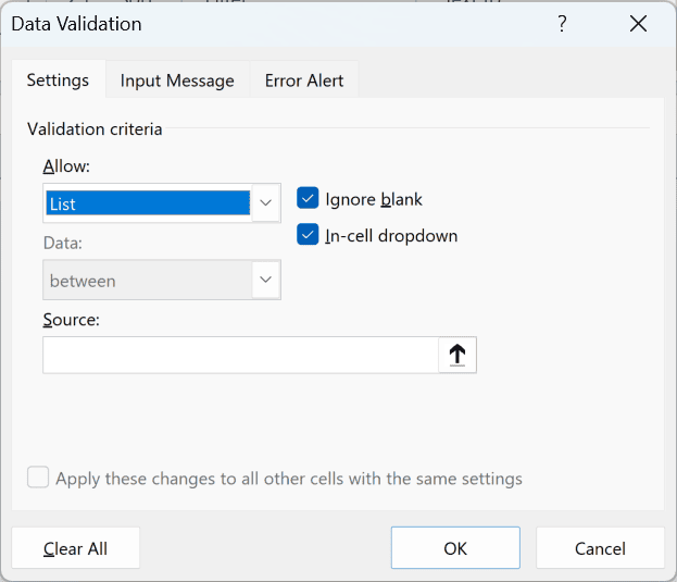
4. Click inside the Source field, and then select cells E2:E3 on the worksheet.

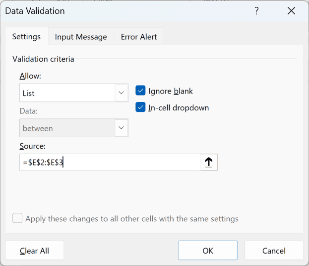
You can also click the range selection icon at the right end of the Source field and select the cells from there.

The reference to these cells (=$E$2:$E$3) is added to the Source field automatically.

5. Click OK.

The above steps create the drop-down in the selected cells using the values in E2:E3 as the source.

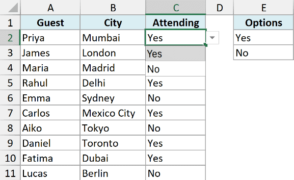
This gives the same result as the previous method. The difference is that if you change the values in E2:E3, the drop-down options update automatically.

If you convert the source cells into an Excel Table, any new option you add below them also shows up in the drop-down.

Also read: Create Data Validation List from Excel Table as Source

Color the Yes/No Drop-Down (Green for Yes, Red for No)

A Yes/No column is much easier to scan when Yes shows up in green and No in red.

The drop-down itself can’t do this, but conditional formatting can. It colors each cell based on the value you pick, and the color updates as soon as you change the value.

Below I have the guest list with the Yes/No drop-down already in C2:C11.

Here are the steps to color the Yes values green:

1. Select the cells with the drop-down (C2:C11).

2. Click the Home tab, and then click Conditional Formatting.

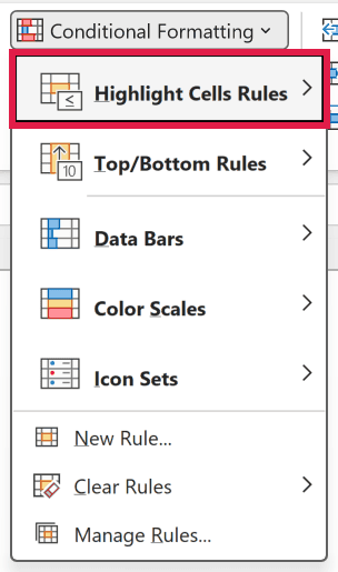
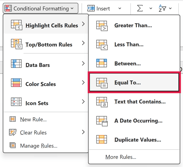
3. Go to Highlight Cells Rules and click Equal To.

4. In the Equal To dialog box, type Yes in the left field.

5. In the drop-down on the right, select Green Fill with Dark Green Text.

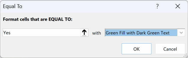
6. Click OK.

Now repeat the same steps for No. Type No in step 4, and select Light Red Fill with Dark Red Text in step 5.

Here is what the result looks like:

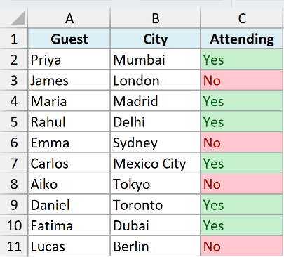
Since this rule checks the value in the cell, it works the same whether you pick the value from the drop-down or copy it in.

If you want to color the entire row instead of just the Yes/No cell, see how to highlight rows based on a cell value.

Count the Yes and No Answers

Once the column is filled in, you’ll usually want to know how many people said Yes and how many said No.

The COUNTIF function does this. In the example file, I’ve entered Yes in E2 and No in E3, and the formula goes in F2.

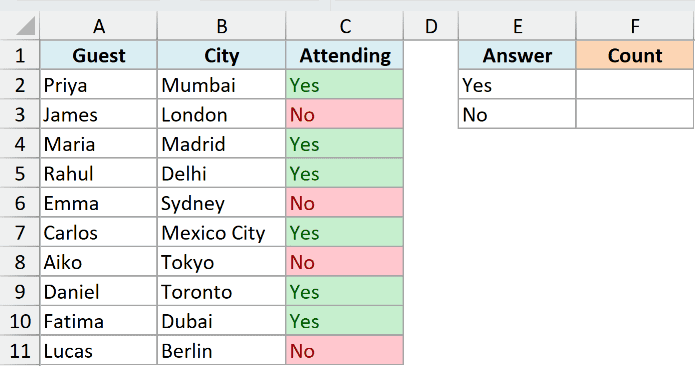
Here is the formula:

=COUNTIF($C$2:$C$11,E2)

Copy it down to F3 to get the count of No answers.

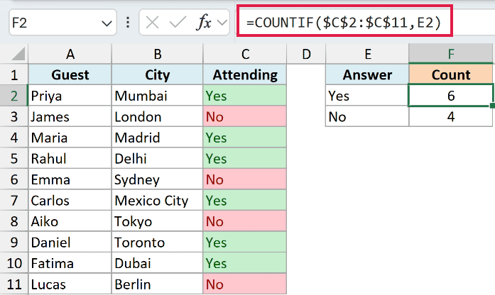
The formula counts the cells in C2:C11 that match the value in E2. So it returns 6 for Yes and 4 for No.

The range is locked with dollar signs so it doesn’t shift when you copy the formula down. COUNTIF isn’t case-sensitive, so “yes” and “Yes” are counted the same.

Copy and Paste the Yes/No Drop-Down List

Drop-down lists can be copied just like cell color or cell formatting.

So, if you already have a Yes/No drop-down in a cell and you want it in other cells, you don’t need to repeat the steps from the previous methods.

You can simply copy the cell that already has the drop-down and paste it over the cells where you want it.

Pro Tip: A normal paste also copies the value and formatting. To copy only the drop-down, use Paste Special (Ctrl + Alt + V) and choose Validation.

Edit the Yes/No Drop-Down List

In case you want to change the values in the drop-down or fix the existing ones, you need to open the Data Validation dialog box and make the changes there.

For example, you may have made a spelling error, or you may want to change the cells the drop-down values are picked from.

In both cases, you’ll have to go back to the Data Validation dialog box to make these changes.

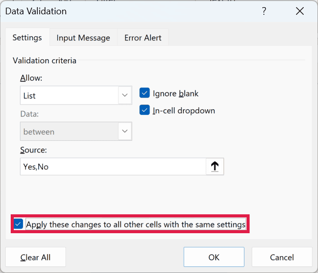
If you copied the drop-down to other cells, check the box that says “Apply these changes to all other cells with the same settings”. This updates every copy in one go.

In this tutorial, I showed you how to create a simple Yes/No drop-down list in Excel, color the answers, and count them.

I hope you found this tutorial useful.

Other Excel tutorials you may also like:

• Drop Down Lists To Show Numbers Between Two Specified Numbers
• Show Symbols in Drop Down Lists in Excel
• Creating Multiple Drop-down Lists in Excel without Repetition
• Display Main and Subcategory in Drop Down List in Excel
• How to Make Multiple Selections in a Drop-Down List in Excel
• Creating a Searchable Drop-Down list in Excel – Step by Step Guide
• How to Create a Dependent Drop-Down List in Excel
• How to Remove Drop-Down List in Excel
• Excel Data Entry Tips