

If you want to find the largest number in a set of values, the MAX function is the fastest way to get it. You point it at your numbers and it returns the biggest one, ignoring any text or blank cells along the way.
MAX returns a single value, but it works right inside dynamic array formulas like =MAX(FILTER(...)) when you need the highest number for a specific group.
In this article, I’ll show you how to use MAX in Excel, from pulling the largest value out of a range to capping a number at a floor and finding the highest amount by category.
MAX Function Syntax
Here is the syntax of the MAX function:
=MAX(number1, [number2], ...)
- number1 – The first number, cell reference, or range you want the largest value from. This one is required.
- [number2], … – Optional extra numbers, references, or ranges. You can add up to 255 in total.
MAX ignores empty cells, text, and the logical values TRUE and FALSE when they sit inside a referenced range. If none of the arguments contain a number, MAX returns 0.
It works in every version of Excel, including Microsoft 365, Excel 2024, 2021, 2019, 2016, and earlier, plus Excel on the web.
When to Use MAX
Use the MAX function when you need to:
- Pull the highest number out of a column, row, or table
- Find the largest value across several ranges that aren’t next to each other
- Get the biggest amount that meets a condition, like the top expense in one category
- Set a floor so a calculation never drops below a certain number
- Find the most recent date in a list
Let me show you a few practical examples of how the MAX function works.
Example 1: Find the Largest Value in a Range
Let’s start with the most common use of MAX, pulling the single highest number out of a list.
Below is a dataset with the days of the week in column A and the number of steps recorded each day in column B.
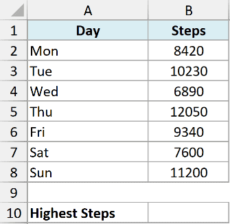
I want to find the highest step count for the week.
Here is the formula:
=MAX(B2:B8)
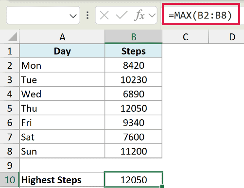
MAX looks through every number in the range B2:B8 and returns the largest one, which is 12,050. It doesn’t matter how the rows are sorted, MAX always finds the biggest value.
Example 2: Use MAX Across Non-Contiguous Ranges
Your numbers won’t always sit in one tidy block. MAX can pull the largest value from several separate ranges at once.
Below is a table of a basketball player’s scoring. Column A has the game number, column B has the points scored in home games, column C has the opponent, and column D has the points scored in away games.
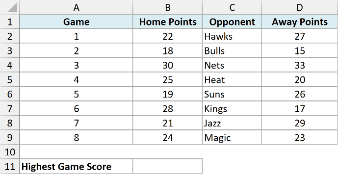
I want the highest single-game points total across both home and away games.
Here is the formula:
=MAX(B2:B9,D2:D9)
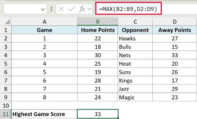
I’ve passed MAX two separate ranges, B2:B9 and D2:D9, with a comma between them. MAX treats them as one big pool of numbers and returns 33, the highest value found in either column.
Pro Tip: You can keep adding more ranges separated by commas, up to 255 arguments in total. This is handy when your values are scattered across columns or even different areas of the sheet.
Example 3: Find the Highest Value That Meets a Condition
Sometimes you don’t want the overall maximum, you want the largest number for one specific category.
Below is an expense log with the date in column A, the expense category in column B, and the amount in column C.
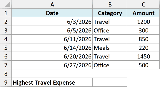
I want the highest Travel expense in the log.
Here is the formula:
=MAX(IF(B2:B7="Travel",C2:C7))
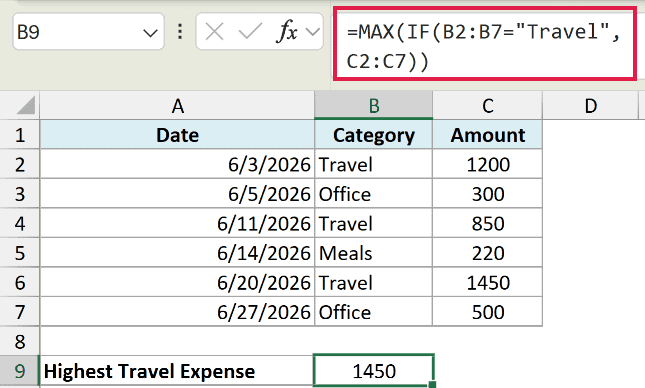
How this formula works:
- The IF part checks every row in B2:B7 to see whether the category is “Travel”.
- For matching rows it returns the amount from column C, and for the rest it returns FALSE.
- MAX then takes the largest number and ignores those FALSE values, giving you 1,450.
In Excel 365 and 2021 you can just type this formula and press Enter. In older versions you need to press Ctrl + Shift + Enter so Excel treats it as an array formula.
Pro Tip: If you have Excel 365, 2021, or 2019, the dedicated MAXIFS function does the same job with a cleaner syntax and no array entry. You give it the max range first, then the range and criteria pair: =MAXIFS(C2:C7,B2:B7,"Travel").
Example 4: Use MAX to Set a Floor at Zero
Here’s a handy trick. You can use MAX to stop a calculation from ever going below a set number, usually zero.
Below is a timesheet with the employee name in column A and the total hours they worked that week in column B. Anything over 40 hours counts as overtime.
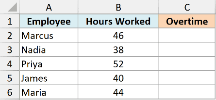
I want the overtime hours for each person, but it should never show a negative number when someone works less than 40 hours.
Here is the formula:
=MAX(0,B2-40)
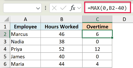
MAX compares two values here, 0 and the result of B2-40.
If the person worked more than 40 hours, B2-40 is positive and MAX returns it. If they worked 40 or fewer hours, B2-40 is zero or negative, so MAX returns 0 instead.
You can copy this formula down the column to get the overtime for everyone on the team.
Example 5: Find the Highest Value by Category With FILTER
If you’re on Excel 365, you can combine MAX with the FILTER function to get the highest value for a group in one clean formula.
Below is a sales table with the product in column A, the region in column B, and the revenue in column C.
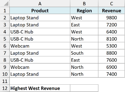
I want the highest revenue figure for the West region.
Here is the formula:
=MAX(FILTER(C2:C10,B2:B10="West"))
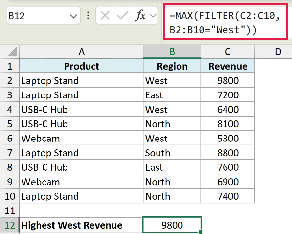
FILTER first pulls out only the revenue values where the region is West. MAX then takes that filtered list and returns the largest one, which is 9,800.
This is where a single-value function like MAX shines. It sits happily inside a dynamic array formula and reduces the filtered list down to the one number you want.
Example 6: Find the Latest Date With MAX
Because Excel stores dates as numbers, MAX works on them just like it does on any other number. That makes it perfect for finding the most recent date.
Below is a list of customer names in column A and the date of their last order in column B.
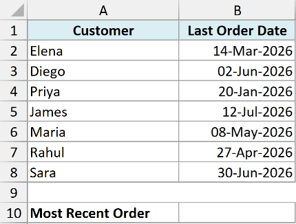
I want to find the most recent order date in the whole list.
Here is the formula:
=MAX(B2:B8)
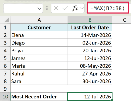
Each date is stored as a serial number, and a later date is a bigger number. So MAX returns the largest one, which shows up as the latest date, 12-Jul-2026 in this case.
Pro Tip: If the result shows up as a number like 46215 instead of a date, the cell just needs formatting. Select it and change the cell format to Date, and it will display correctly.
Tips & Common Mistakes
- MAX ignores text and blank cells. If a range has text labels or empty rows mixed in with your numbers, MAX skips them and still returns the largest number. You don’t need to clean the range first.
- It also ignores TRUE and FALSE inside a referenced range. If you actually want logical values counted as 1 and 0, use the MAXA function instead of MAX.
- Typed-in values behave differently from referenced ones. Logical values and numbers-as-text that you type straight into the formula (like
=MAX(TRUE,5)) do get counted, but the same values sitting in a referenced cell are ignored. - Use MAXIFS for conditions. For the highest value that meets one or more conditions, the MAXIFS function (Excel 365, 2021, 2019) is cleaner than a MAX IF array formula. It takes the max range first, then range and criteria pairs.
- A surprise 0 usually means no numbers. If your arguments contain no numbers at all, MAX returns 0 rather than an error. That often means the range you pointed at holds only text or blank cells.
- Need the second or third highest? MAX only ever returns the single biggest value. To get the second largest value or any Nth highest number, use the LARGE function instead.
That covers the MAX function in Excel. We looked at finding the largest value in a range, pulling the max from separate ranges, getting the highest value for a condition, setting a floor at zero, combining MAX with FILTER, and finding the latest date.
It’s a small function that does a lot once you know these tricks. I hope you found this article helpful.
Other Excel Articles You May Also Like:
