

If you want to round a number to a set number of decimal places or to the nearest 10, 100, or 1000, the ROUND function is what you need. It changes the actual value, not just how the number looks on screen.
In Excel 365, you can also feed ROUND a range and the results spill into the cells below. In this article, I’ll show you how to use ROUND with plenty of practical examples.
ROUND Syntax
Here is the syntax of the ROUND function:
=ROUND(number, num_digits)
- number – the number you want to round.
- num_digits – how many digits you want to round the number to. A positive value rounds to decimal places, 0 rounds to a whole number, and a negative value rounds to the left of the decimal point.
Both arguments are required.
When to Use ROUND in Excel
Use the ROUND function when you need to:
- Round prices or amounts to a fixed number of decimal places.
- Clean up long decimals that come out of a calculation.
- Round large numbers to the nearest 10, 100, or 1000 for a summary.
- Make the stored value match what you actually want, not just the display.
Let me show you a few practical examples of how this works.
Example 1: Round to Two Decimal Places (Currency)
Let’s start with a common one, rounding prices to two decimal places.
Below is a dataset with a list of items and their prices after a currency conversion, which left a lot of extra decimals.
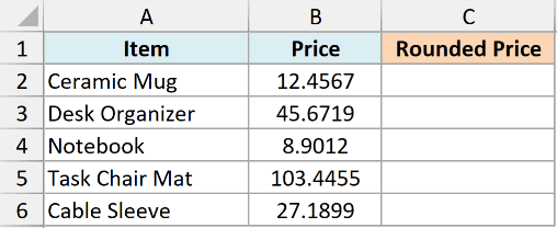
I want to round every price to two decimal places so it reads as a clean currency amount.
Here is the formula:
=ROUND(B2:B6, 2)
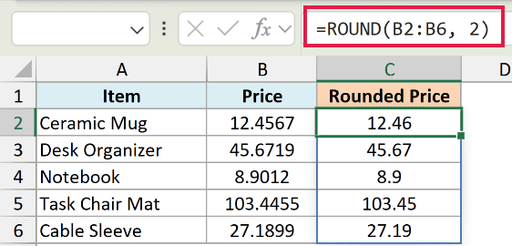
Since num_digits is 2, ROUND keeps two digits after the decimal point. So 12.4567 becomes 12.46 and 45.6719 becomes 45.67.
I fed ROUND the whole range B2:B6 in one go, so in Excel 365 the results spill down automatically. You don’t need to copy the formula to each row.
Pro Tip: On older versions of Excel that don’t support spilling, write =ROUND(B2, 2) in the first cell and drag it down the column.
Example 2: Round to the Nearest Whole Number
Here’s another common scenario, rounding to whole numbers.
Below is a dataset with a list of packages and their measured weights in kilograms.
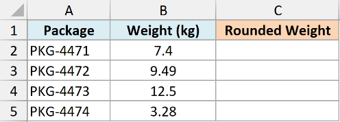
I want to round each weight to the nearest whole kilogram.
Here is the formula:
=ROUND(B2:B5, 0)
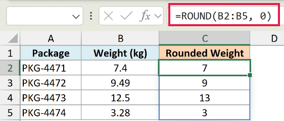
When you use 0 as the num_digits argument, ROUND rounds to the nearest whole number. So 7.4 becomes 7 and 9.49 becomes 9.
Notice that 12.5 rounds up to 13. ROUND rounds a trailing .5 away from zero, so exact halves always go up (or down, for negative numbers).
If you instead want to always drop the decimals and keep only the whole part, the INT function does that.
Example 3: Round to the Nearest Thousand (Negative Digits)
Now let’s look at something a lot of people don’t know ROUND can do.
Below is a dataset with a list of cities and their populations. The exact figures are too detailed for a quick summary.
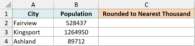
I want to round each population to the nearest thousand.
Here is the formula:
=ROUND(B2:B4, -3)
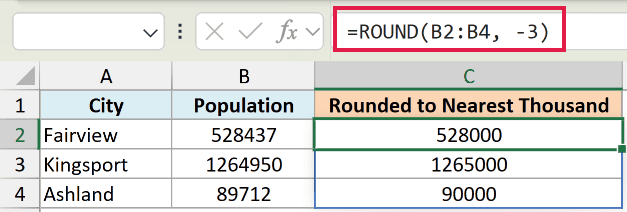
A negative num_digits rounds to the left of the decimal point. Here, -3 rounds to the nearest thousand, so 528437 becomes 528000 and 1264950 becomes 1265000.
Pro Tip: Use -1 to round to the nearest 10, -2 for the nearest 100, and -3 for the nearest 1000. To display big numbers in a summary without changing them, you can also format numbers to show in millions.
Example 4: Round a Calculated Total to Avoid Penny Drift
Let’s step it up with something I use on almost every invoice.
Below is a dataset with a price and quantity for each item. The line total needs 8.25% tax added, which produces long decimals.
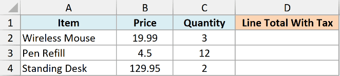
I want each line total rounded to the cent so the invoice adds up exactly.
Here is the formula:
=ROUND(B2:B4*C2:C4*1.0825, 2)
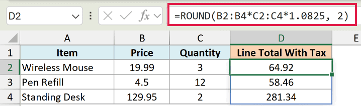
The formula multiplies price by quantity, then by 1.0825 to add the tax, and rounds the result to two decimals. So 19.99 times 3 with tax gives 64.92.
This matters when you sum the column. If each line is rounded to an exact cent, the total reconciles perfectly instead of drifting a penny off from what people see.
Example 5: ROUND vs. Changing the Cell Format
This is the difference that trips up the most people, so let’s look at it directly.
Below is a dataset with two tasks and the hours spent on each. Both cells show 10 because they’re formatted to zero decimals, but the real values are 10.4.
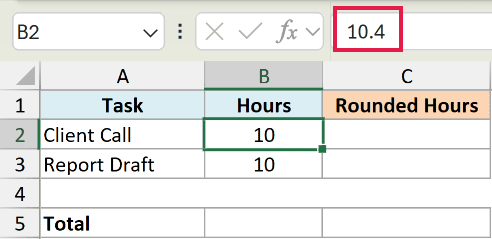
I want the stored values to actually be whole numbers, not just look like whole numbers.
Here is the formula:
=ROUND(B2:B3, 0)
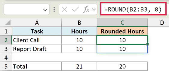
Formatting only changes the display. The cell still holds 10.4, so a SUM of the two formatted cells returns 20.8, which shows as 21. It looks like 10 plus 10 equals 21.
ROUND changes the real value to 10, so the sum is a true 20. Use ROUND when the math has to match what you see, and use formatting when you only care about the display. If Excel is trimming your decimals on its own, here’s how to stop Excel from rounding numbers.
Example 6: ROUND vs. ROUNDUP, ROUNDDOWN, and MROUND
Finally, let’s see how ROUND compares to its close cousins.
Below is a dataset with a single value, 8.6, that we’ll pass through each function.
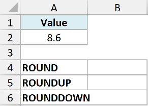
I want to see how each rounding function treats the same number.
Here is the ROUND formula:
=ROUND(A2, 0)
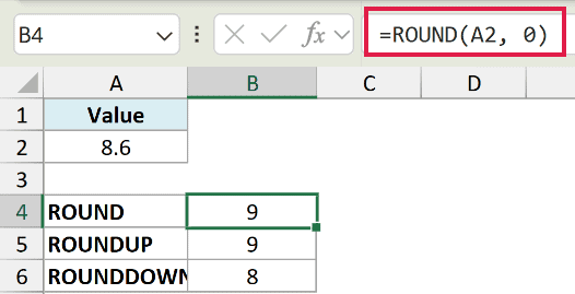
ROUND goes to the nearest whole number, so 8.6 becomes 9 because it’s past the halfway point.
Here is the ROUNDUP formula:
=ROUNDUP(A2, 0)
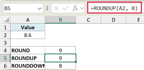
ROUNDUP always rounds away from zero, so it also returns 9 here. But it would return 9 even for 8.1, where ROUND would give 8.
Here is the ROUNDDOWN formula:
=ROUNDDOWN(A2, 0)
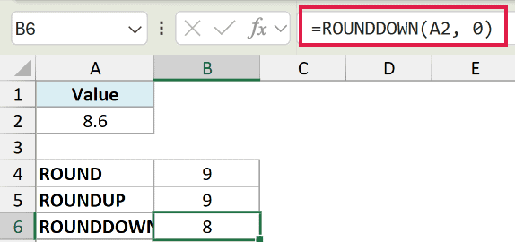
ROUNDDOWN always rounds toward zero, so 8.6 becomes 8 even though it’s past the halfway point.
Pro Tip: To round to the nearest multiple of a number (like the nearest 5), use the MROUND function instead. For example, =MROUND(8.6, 5) returns 10.
Tips & Common Mistakes
- ROUND rounds half away from zero. A trailing .5 always moves away from zero, so 2.5 becomes 3 and -2.5 becomes -3. This is not the “round half to even” (banker’s rounding) some tools use.
- Negative digits round to the left of the decimal. -1 rounds to the nearest 10, -2 to the nearest 100, and -3 to the nearest 1000. It’s an easy way to round big numbers for a summary.
- ROUND changes the value, formatting only changes the display. If you only reduce the decimals shown, the full value is still stored and used in calculations. Use ROUND when the underlying number has to change.
- Feed a range to spill in Excel 365. A formula like =ROUND(B2:B6, 2) spills down the column, so you don’t need to fill it into each cell one by one.
That covers the main ways to use the ROUND function in Excel, from rounding currency to two decimals, to rounding big numbers to the nearest thousand with negative digits.
The key thing to remember is that ROUND changes the actual value. That’s exactly what you want when the math needs to match what’s on screen.
Other Excel Articles You May Also Like:
