

If you want to convert minutes into hundredths in Excel, the trick is to turn each value into decimal hours.
This is what payroll systems use, where
- 15 minutes becomes 0.25
- 30 minutes becomes 0.50
- 45 minutes becomes 0.75, and so on.
The reason people get stuck is that the right formula depends on how your data is stored. A plain number like 90 needs one approach, and a real Excel time like 1:30 needs another.
In this article, I’ll show you how to convert minutes to hundredths in both situations, plus how to show just two decimals using cell formatting or the ROUND function.
What “Hundredths” Actually Means Here
When someone says they need minutes in hundredths, they almost always mean decimal hours.
Instead of writing one hour and thirty minutes, you write 1.50. Instead of forty-five minutes, you write 0.75. The minutes get expressed as a fraction of an hour, shown to two decimal places.
This matters because most payroll and billing systems can only add up decimal hours, not the hours-and-minutes format. So 90 minutes of work needs to show up as 1.50 hours, not as 1:30.
The math behind it is simple. There are 60 minutes in an hour, so you divide the minutes by 60 to get the decimal value.
Which formula you reach for depends on how the minutes are stored. Here is the quick version, and the sections below walk through each one:
| If your minutes are stored as… | Formula | Example |
|---|---|---|
| A plain number (like 90) | =A2/60 | 90 → 1.50 |
| A real Excel time (like 1:30) | =A2*24 | 1:30 → 1.50 |
Method 1: Convert Minutes Stored as a Plain Number
Let’s start with the most common situation. Your minutes are sitting in a cell as a regular number, like 90 or 45.
In this case, you divide the value by 60 to get decimal hours. Let me show you how it works.
Below is a dataset with the number of minutes each person worked on a task, listed in column A.
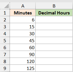
Here is the formula:
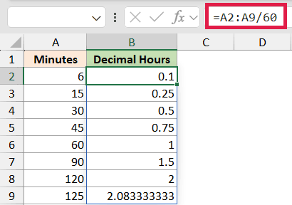
=A2:A9/60
How does this formula work?
The range A2:A9 holds the minutes, and I divide it by 60 because there are 60 minutes in one hour.
Because the formula points at the whole range, the result spills down the column on its own. You type it once in cell B2 and Excel fills the rest, with no dragging or copying needed.
So 90 minutes returns 1.5, which means one and a half hours, and 45 minutes returns 0.75.
Here is what you get when you run this on a few values:
- 6 minutes becomes 0.10
- 45 minutes becomes 0.75
- 60 minutes becomes 1.00
- 90 minutes becomes 1.50
- 125 minutes becomes 2.083333
That last result shows a problem. The value runs to many decimal places, which is not what you want for payroll.
I’ll show you two ways to clean that up further down: first with cell formatting in Method 3, then with the ROUND function in Method 4.
Method 2: Convert a Value Stored as a Real Excel Time
Now let’s look at the other situation. Sometimes the value is a genuine Excel time, like 1:30 typed into a cell, not a plain number.
Here you multiply the value by 24 instead of dividing by 60. Let me explain why that works.
Below is a dataset with the same employees, but this time the duration is stored as an actual time value.
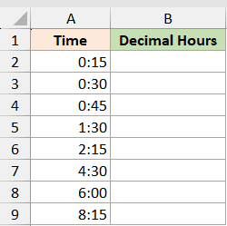
Here is the formula:
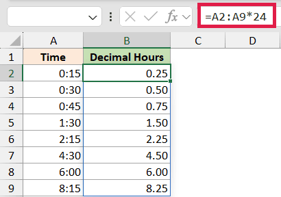
=A2:A9*24
How does this formula work?
Excel stores time as a fraction of a day, where a full day equals 1. So one hour is 1/24, and the time 1:30 is actually stored as 0.0625 behind the scenes.
When I multiply that stored value by 24, I scale it back up to hours. So 1:30 gives 1.5, and 8:15 gives 8.25.
Pointed at the range A2:A9, the formula spills a decimal hour for every row at once, so you only enter it in the top cell.
There is one catch. After you enter this formula, Excel often copies the time format onto the spilled result cells, so they show something odd instead of clean numbers.
To fix this, select the result cells, go to the Home tab, and set the number format to Number or General. Now the value displays as 1.50 the way you expect.
Method 3: Show Two Decimals with Cell Formatting (Keeps Full Precision)
Remember the long decimals from Method 1, like 2.083333 for 125 minutes? The easiest way to tidy those up is to divide by 60 as before, then simply format the cells to show two decimals.
Formatting changes only what you see on screen. The backend value in the cell in Excel does not change.
We’re back to the same minutes sitting in column A (A2:A9), values like 90 and 125, and the goal is to display each one as decimal hours with two decimal places.
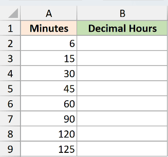
Start with the same formula as Method 1:
=A2:A9/60
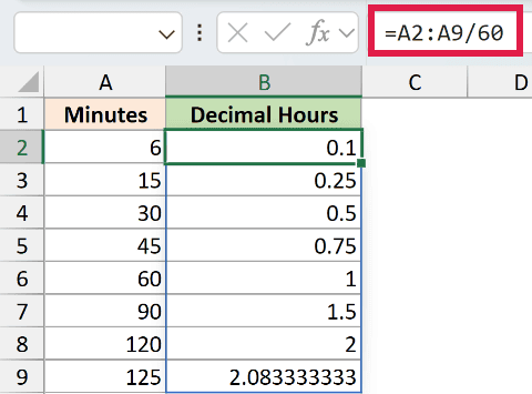
This spills the decimal hours down the column, and you can see some values still run long. Now you format those cells to clean up the display.
Here are the steps to show two decimals with cell formatting:
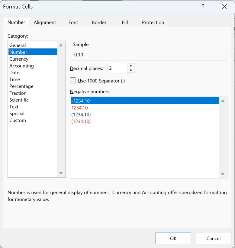
- Select the result cells that hold the decimal hours (the spilled range in column B).
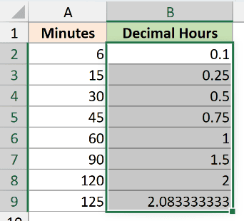
- On the Home tab, click the small arrow in the corner of the Number group to open the Format Cells dialog, or just press Control + 1.
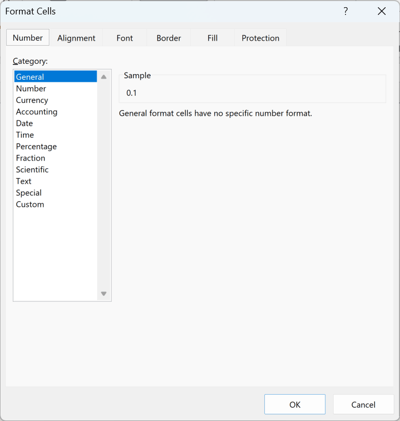
- Pick Number on the left, set Decimal places to 2, and click OK.
Now each cell shows a clean two-decimal value, so 125 minutes reads as 2.08. But nothing about the stored number changed.
The formula bar still shows the plain =A2:A9/60, so Excel holds on to the full 2.083333 whenever it adds these up.
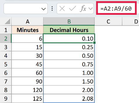
That’s the whole advantage. The number you see is tidy, and the number Excel stores stays exact, so summing the column gives you the most accurate total.
Method 4: Round the Result to Two Decimals (Hundredths)
In Method 3, formatting tidied up how that long decimal looks, but the actual value stayed at 2.083333. Sometimes you need the stored value itself to be just two decimals, and that is where ROUND comes in.
To keep it to two decimal places, wrap your formula inside the ROUND function. The word hundredths is just another way of saying two decimal places.
We’re back to the same minutes sitting in column A (A2:A9), values like 90 and 125, and this time the goal is to convert them to decimal hours but keep only two decimal places.
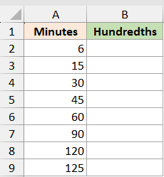
For minutes stored as a plain number, use this:
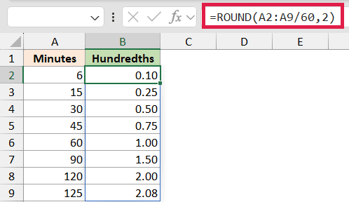
=ROUND(A2:A9/60,2)
If your value is a real Excel time instead, use this version:
=ROUND(A2:A9*24,2)
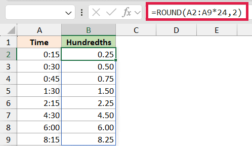
How does this formula work?
The ROUND function takes two things. The first is the number you want to round, and the second is how many decimal places you want.
I put 2 as the second part because hundredths means two decimal places. So 125 minutes, which was 2.083333, now becomes a clean 2.08.
Just like in Method 1, pointing ROUND at the range A2:A9 spills the rounded result down every row in one go.
Unlike the formatting in Method 3, this changes the stored value itself, not just how it looks. So the 2.08 you see is the exact number Excel uses everywhere else.
Formatting vs ROUND: Which Should You Use?
Both methods land on 2.08, so which one is right? It comes down to what happens to that number next.
Cell formatting keeps the exact value and only cleans up the display. That gives you the most accurate totals when you add up a column, because Excel sums the full values behind the scenes.
ROUND actually changes the stored value to two decimals. That’s what you want when the figure gets paid out, exported, or fed into another formula, so what people see is exactly what gets used.
Pro Tip: Use cell formatting when the decimal hours are an in-between value you will sum or calculate with. Use ROUND when that two-decimal number is the final figure that feeds pay or another formula.
A Quick Reference Table for Common Minutes
It helps to keep a small table handy so you can sanity-check your formulas. Here is how the common minute marks map to their hundredths value.
| Minutes | Decimal (Hundredths) |
|---|---|
| 6 | 0.10 |
| 15 | 0.25 |
| 30 | 0.50 |
| 45 | 0.75 |
| 60 | 1.00 |
| 90 | 1.50 |
If your formula returns one of these numbers for the matching minutes, you know it is working correctly.
Going the Other Way: Hundredths Back to Minutes
Sometimes you need the reverse. You have decimal hours and want to get back to minutes.
For that, you multiply the decimal value by 60. So 1.5 hours multiplied by 60 gives you 90 minutes, and 0.75 multiplied by 60 gives 45.
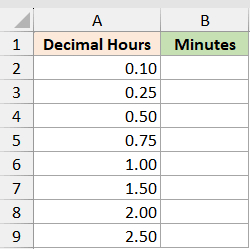
For this one, your decimal hours sit in column A (A2:A9), values like 1.5 and 0.75, and the goal is to turn each one back into plain minutes. Here is the formula:
=A2:A9*60
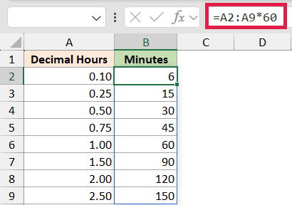
As with the other methods, the ranged formula spills a minute value for every row automatically. This is handy when someone hands you a timesheet in decimal hours and your own system still wants plain minutes.
Things to Keep in Mind
- Know how your data is stored before picking a formula. Divide by 60 when the minutes are a plain number. Multiply by 24 when the value is a real Excel time. Using the wrong one gives you a value that is off by a large factor.
- Watch the cell format after multiplying a time by 24. Excel often keeps the time format on the result, so set the cell to Number or General to see a clean decimal.
- Pick formatting or ROUND based on what the number feeds. Cell formatting keeps the most accurate totals while tidying the display. ROUND is for when the two-decimal figure itself gets paid or exported, so what people see is what gets used.
- If you only need a display value and not a calculation, you can also format the result with the TEXT function, like =TEXT(A2:A9/60,”0.00″). Just remember the output becomes text, so it will not add up in later formulas.
In this article, I showed you how to convert minutes to hundredths in Excel, whether your data is a plain number or a real Excel time, plus how to show two decimals with cell formatting or ROUND, and how to reverse it.
I hope you found this article helpful.
Other Excel Articles You May Also Like:
