TEXT Function in Excel (6 Examples)

If you want to take a number, a date, or a time in Excel and show it in a specific format, the TEXT function is what you’re looking for.

It lets you turn a value like 1234567 into “1,234,567” or a date into “15-Jul-2026”.

The trick is knowing which format code to use, and that’s the part most people get stuck on. In this article I’ll walk you through the TEXT function with real examples, and give you a reference table of the format codes you’ll actually use.

TEXT Function Syntax

The TEXT function converts a number into text and displays it using a format code that you supply.

=TEXT(value, format_text)

Input Arguments

• value: The number, date, or time you want to convert. This has to be a numeric value (a number, or a date/time, which Excel stores as a number).
• format_text: A format code in double quotes that tells Excel how to display the value, like "0.00" or "dd-mmm-yyyy".

Both arguments are required. The result is always text, which matters later, so keep it in mind.

Excel TEXT Function Format Codes (Reference Table)

The whole job of the TEXT function is choosing the right format code. Here are the ones you’ll reach for most often.

Format code	What it does	Example input	Example result
0	Shows a digit, and pads with zeros if needed	42	42
0.00	Shows two decimal places	8.5	8.50
#	Shows a digit only if it’s significant	8.50	8.5
#,##0	Adds thousands separators	1234567	1,234,567
$#,##0.00	Currency with two decimals	2500.5	$2,500.50
0.0%	Percentage with one decimal	0.4567	45.7%
00000	Leading zeros (fixed width)	42	00042
dd-mmm-yyyy	Day, short month, year	a date	15-Jul-2026
mmmm	Full month name	a date	July
dddd	Full day name	a date	Wednesday
h:mm AM/PM	12-hour time	a time	1:29 PM

One thing worth knowing early: format codes aren’t case sensitive for dates and times, so dd-mmm-yyyy and DD-MMM-YYYY do the same thing.

Pro Tip: If you’re not sure what a format code looks like, open Format Cells (Ctrl + 1), pick a format under the Custom category, and copy the code from the Type box. Any code that works there works inside TEXT too.

Example 1: Format a Date with the TEXT Function

Let’s start with dates, which is where most people first meet the TEXT function. It’s also the most reliable way to convert a date to text in Excel while keeping the exact look you want.

Below I have a list of dates in column A, and I want to show each one as “15-Jul-2026” (day, short month name, full year) in column B.

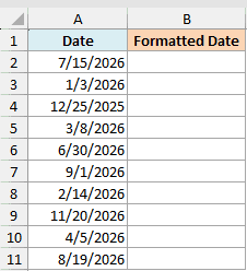
Here is the formula:

=TEXT(A2:A11,"dd-mmm-yyyy")

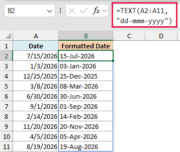
Because I passed the whole range A2:A11 in one go, the formula spills the results down column B automatically. You type it once in B2 and Excel fills the rest. No dragging, no Ctrl+Shift+Enter.

The format code dd-mmm-yyyy is doing the work here. dd is the two-digit day, mmm is the short month name, and yyyy is the four-digit year.

If you want to explore more ways to change the date format in Excel, I have a separate guide on that.

Pro Tip: The spilling form (a single formula on a range) needs Microsoft 365 or Excel 2021. On older versions, put =TEXT(A2,”dd-mmm-yyyy”) in B2 and copy it down.

Example 2: Add Thousands Separators and Currency with TEXT

Now let’s format some numbers so they’re easier to read.

Below I have raw sales figures in column A, and I want to show them with thousands separators in column B, so 1234567 reads as 1,234,567.

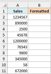
Here is the formula:

=TEXT(A2:A11,"#,##0")

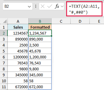
The #,##0 code adds a comma every three digits. The # shows a digit only when it’s needed, and the 0 makes sure at least one digit always shows, even for a value like 0.

If you want a dollar sign and two decimal places, add them to the format code instead.

=TEXT(A2:A11,"$#,##0.00")

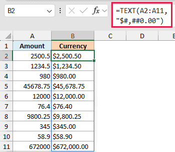
This turns 2500.5 into $2,500.50. The $ prints the dollar sign, and .00 forces exactly two decimal places. The same idea lets you format large numbers to show in millions when the raw figures get too long to read.

Example 3: Show Numbers as Percentages with TEXT

Let’s look at percentages next, since this is one people often get wrong.

Below I have decimal values in column A, like 0.4567, and I want to show them as percentages in column B.

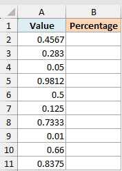
Here is the formula:

=TEXT(A2:A11,"0.0%")

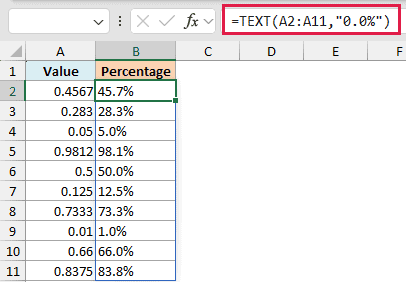
The % code multiplies the value by 100 and adds the percent sign, so 0.4567 becomes 45.7%. The 0.0 part controls the decimals, so you get one digit after the point.

Want no decimals? Use "0%" instead, and 0.4567 rounds to 46%.

Example 4: Add Leading Zeros to IDs and Zip Codes with TEXT

Here’s a common one. Excel drops leading zeros from numbers, so an ID like 00042 shows up as just 42. The TEXT function fixes that.

Below I have employee IDs in column A that lost their leading zeros, and I want every ID to be five digits in column B.

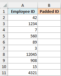
Here is the formula:

=TEXT(A2:A11,"00000")

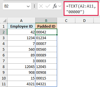
Each 0 in the format code is a fixed slot. Five zeros means the result is always five digits, so 42 becomes 00042 and 1234 becomes 01234. This is handy for zip codes and product codes too.

There are a few other ways to add leading zeros in Excel if you’d rather not use a formula.

Example 5: Format a Phone Number with TEXT

You can also use TEXT to turn a plain string of digits into a formatted phone number.

Below I have 10-digit numbers in column A, and I want them shown as (123) 456-7890 in column B.

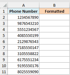
Here is the formula:

=TEXT(A2:A11,"(###) ###-####")

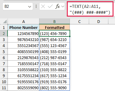
The format code places each digit into a slot, adds the parentheses around the area code, and drops a dash before the last four digits. So 1234567890 becomes (123) 456-7890.

Example 6: Combine TEXT with the & Operator to Build a Label

The TEXT function is really useful when you join a formatted value into a sentence. If you try to join a raw number or date with &, Excel shows the ugly underlying value. TEXT lets you control exactly how it looks.

Below I have order totals in column A and dates in column B, and I want a clean label in column C like “Total: $1,234.50 on 15-Jul-2026”.

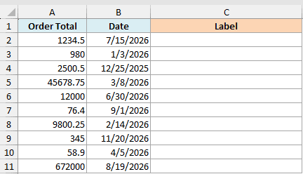
Here is the formula:

="Total: "&TEXT(A2:A11,"$#,##0.00")&" on "&TEXT(B2:B11,"dd-mmm-yyyy")

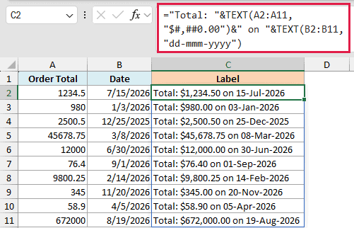
Each TEXT wraps its value in a format code, and the & glues the pieces together with the plain text in between. Without TEXT, that date would show up as a serial number like 46218 instead of a readable date.

Tips and Common Mistakes

• The result is text, not a number. This is the big one. A TEXT result can’t be summed or used in math. If you run =SUM() on a column of TEXT results, you’ll get 0. Keep your real numbers in one column and use TEXT only for display.
• mm means month or minutes depending on where it sits. On its own, or next to dd/yyyy, mm is the month. Right after hh, it’s minutes. So hh:mm is hours and minutes, not hours and months.
• Format codes go in double quotes. =TEXT(A2,"0.00") works. Leaving out the quotes gives an error.
• TEXT doesn’t change the real value. It only changes how the value looks in the new cell. The original number in column A is untouched.

Wrapping Up

The TEXT function is one of those small tools that makes your spreadsheets a lot more readable, whether you’re formatting dates, adding thousands separators, or building clean labels.

Once you get comfortable with the format codes in the reference table above, you’ll use it all the time.

I hope you found this tutorial helpful.

Other Excel Articles You May Also Like:

• Excel CONCATENATE Function
• How to Convert Numbers to Text in Excel
• How to Format Phone Numbers in Excel?
• Custom Number Formatting in Excel