LINEST Function in Excel

If you want to fit a straight line to your data and get the slope, the intercept, and how good the fit actually is, the LINEST function is what you’re after.

It runs a least-squares regression and hands back the numbers behind the line.

LINEST returns a whole array of numbers, not just one. In Microsoft 365, that array spills into the cells below and to the right on its own.

In this article I’ll show you how to use LINEST, starting with a simple slope and intercept and working up to full regression stats, multiple predictors, and a quadratic curve.

LINEST Function Syntax

Here is the syntax of the LINEST function:

=LINEST(known_y's, [known_x's], [const], [stats])

• known_y’s – required. The dependent values you’re trying to explain or predict (the y column).
• known_x’s – optional. One or more ranges of independent values (the x columns). Leave it out and Excel uses {1,2,3,…}.
• const – optional. TRUE or omitted lets Excel calculate the intercept normally. FALSE forces the intercept to 0.
• stats – optional. TRUE returns the full grid of regression statistics. FALSE or omitted returns just the coefficients and the intercept.

If you give LINEST only the y values, it assumes the x values are 1, 2, 3, and so on. That’s handy for a simple trend over numbered periods.

The const argument decides whether the line gets its own starting point. Leave it out (or use TRUE) and Excel calculates the intercept. Use FALSE to pin it to 0.

The stats argument decides how much you get back. Leave it out and you get one row of coefficients. Set it to TRUE and you get a five-row grid of statistics.

LINEST works in Excel for Microsoft 365, Excel 2024, 2021, 2019, and 2016, including the Mac versions.

When to Use LINEST for Linear Regression

Use the LINEST function when you need to:

• Get the slope and intercept of a best-fit line without reading them off a chart trendline label.
• Measure how well a line fits with R-squared, standard errors, the F statistic, degrees of freedom, and the sums of squares.
• Fit a multiple regression with several independent variables in one formula.
• Use the fitted coefficients to estimate an outcome for a new input.
• Fit a curved relationship by feeding LINEST powers of x.

Let me show you a few practical examples of how this works.

Example 1: Return the Slope and Intercept

Let’s start with the simplest case: a straight line through two columns of data.

Below is a small table of e-bike courier routes. Column A has the route distance in kilometers, and column B has the battery percentage used on that route.

There are eight routes in A2:B9.

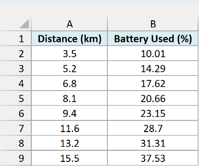
I want to fit a line so I can see how much battery each extra kilometer costs, plus the baseline drain.

Here is the formula:

=LINEST(B2:B9,A2:A9)

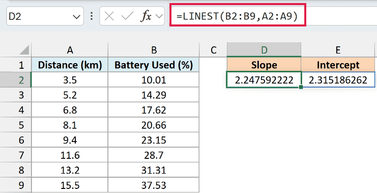
This spills two numbers into two cells. The left cell shows the slope, about 2.2476, and the right cell shows the intercept, about 2.3152.

So each kilometer uses roughly 2.25% more battery, and a route starts at about 2.32% even before any distance. The line is battery = 2.2476 × distance + 2.3152.

Notice you didn’t drag anything or press Ctrl+Shift+Enter. You typed one formula in one cell and both numbers appeared side by side.

Pro Tip: The slope always lands in the left cell and the intercept in the right. If you usually write the line as y = a + bx, that order can feel backwards.

Important: If you see a #SPILL! error, something is blocking the output. Clear the cells below and to the right, and keep the formula out of an Excel Table.

Important: Excel 2019 and 2016 don’t spill. Select the whole output range, type the formula, and press Ctrl+Shift+Enter. This works for every example here except 6 and 7.

Pro Tip: Need only one number? The SLOPE and INTERCEPT functions are simpler than reading a LINEST grid. Here’s how to find the slope in Excel.

Example 2: Get the Full LINEST Output (Regression Statistics)

Now let’s ask LINEST for the full picture by setting the last two arguments to TRUE.

Below is a table of student study logs. Column A has the hours studied, and column B has the exam score out of 100, across ten students in A2:B11.

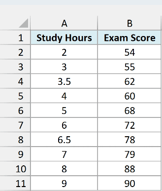
I want the slope and intercept along with every statistic that tells me how trustworthy the line is.

Here is the formula:

=LINEST(B2:B11,A2:A11,TRUE,TRUE)

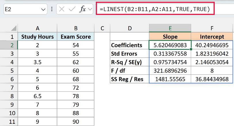
With stats set to TRUE, the result spills into a 5-row by 2-column block. Here is what each cell holds for this data:

Output row	Left cell	Right cell
Row 1	Slope (5.6205)	Intercept (40.2495)
Row 2	Standard error of the slope (0.3134)	Standard error of the intercept (1.8232)
Row 3	R-squared (0.9757)	Standard error of the y estimate (2.1461)
Row 4	F statistic (321.69)	Degrees of freedom (8)
Row 5	Regression sum of squares (1481.56)	Residual sum of squares (36.84)

The one to look at first is R-squared. Here it’s 0.9757, so about 98% of the variation in exam scores is explained by the study hours.

Excel doesn’t label any of these cells for you. It just drops the numbers in a grid, so keep the table above handy when you read one.

In the example file, I’ve added the row labels in column D myself to make the grid easier to read.

Example 3: Extract Just R-Squared with INDEX

Sometimes you only want one number out of that grid. Let’s pull R-squared on its own.

Below is a table of monthly ad campaigns. Column A has the ad spend in dollars, and column B has the sales in dollars, over eight months in A2:B9.

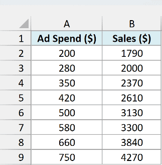
I want a single cell showing how well the ad spend explains sales, without the rest of the stats grid cluttering the sheet.

Here is the formula:

=INDEX(LINEST(B2:B9,A2:A9,TRUE,TRUE),3,1)

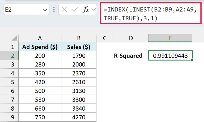
This returns 0.9911, so about 99% of the change in sales tracks with the ad spend.

R-squared sits in row 3, column 1 of the LINEST output, and that’s exactly the cell the INDEX function grabs here.

LINEST still builds the whole 5-by-2 array in memory, but INDEX pulls out only the cell you asked for.

Pro Tip: Use the same trick for any single statistic. INDEX(LINEST(…),1,1) gives the slope, INDEX(LINEST(…),1,2) gives the intercept, and row 3, column 1 gives R-squared.

Example 4: Force the Intercept Through Zero

There are times when the line has to pass through the origin. Let’s tell LINEST to force the intercept to 0.

Below is a table of hourly-wage timesheets. Column A has the hours worked, and column B has the pay in dollars, over eight paychecks in A2:B9.

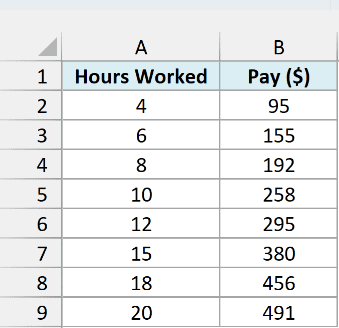
Zero hours worked has to mean zero pay, so I want a line pinned to the origin. I set the const argument to FALSE.

Here is the formula:

=LINEST(B2:B9,A2:A9,FALSE,TRUE)

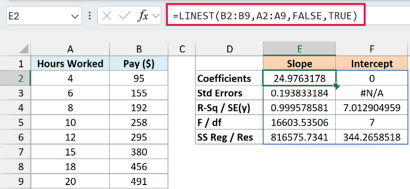
The slope comes back as 24.9763, and the intercept cell now shows 0 because we forced it there. R-squared is 0.9996.

Look at row 2, column 2. The standard error of the intercept shows #N/A.

That isn’t a broken formula. With the intercept forced to 0, there’s nothing to estimate an error for, so LINEST returns #N/A on purpose.

So the fitted line is pay = 24.9763 × hours worked, meaning the pay comes to about $25 an hour with no fixed offset.

Important: With const set to FALSE, LINEST calculates R-squared differently, so it usually comes out higher. Don’t compare it with the R-squared of a normal fit.

Pro Tip: Only set const to FALSE when the logic truly demands a zero start. Forcing it just to bump up R-squared can make the model misleading.

Example 5: Run a Multiple Linear Regression

LINEST isn’t limited to one predictor. Let’s fit a model with three of them at once.

Below is a table of twelve food-delivery runs in A2:E13. Column A has the run ID, and column B has the route distance in kilometers.

Column C has the number of apartment-building stops, column D has the minutes of heavy rain, and column E has the total delivery time in minutes.

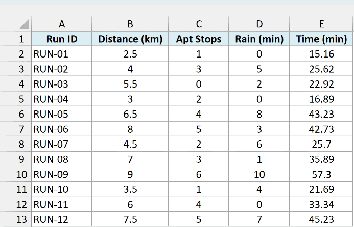
I want to see how much each of the three factors adds to the delivery time on its own.

Here is the formula:

=LINEST(E2:E13,B2:D13,TRUE,TRUE)

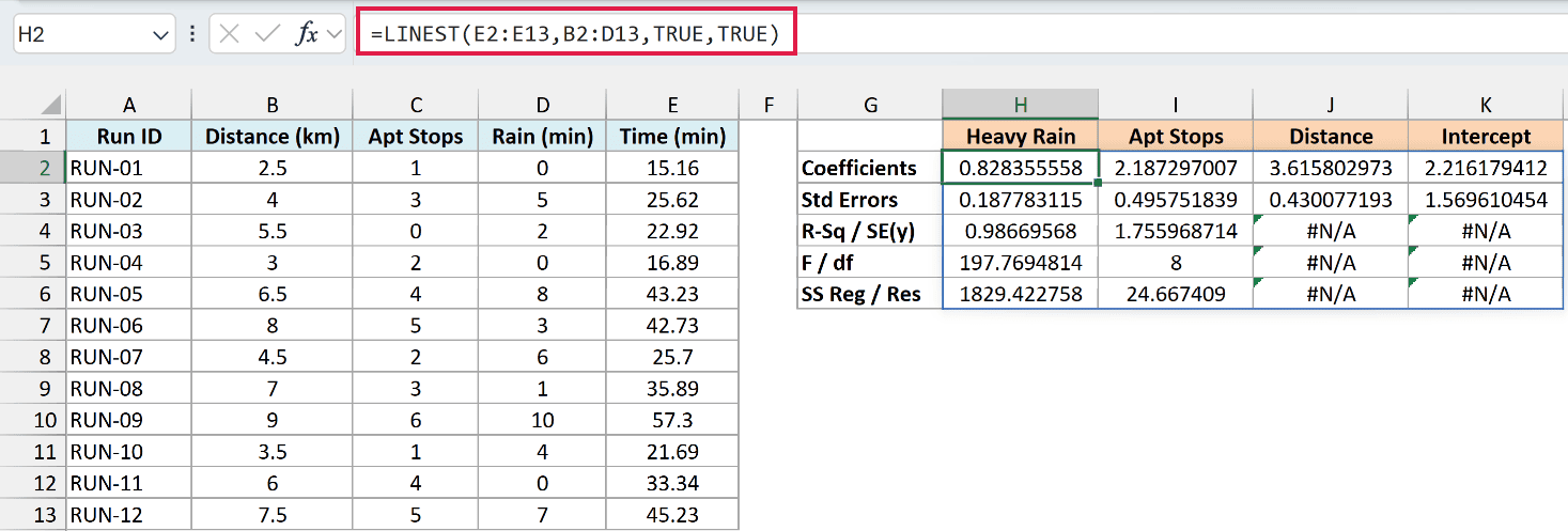
With three predictors, the result spills into a 5-row by 4-column block. The first row holds the three coefficients and then the intercept.

Rows 3 to 5 use only the first two columns. The other cells in those rows show #N/A, and that’s normal, not a data error.

Here’s the catch that trips everyone up: the coefficients come back in reverse column order. Reading row 1 from left to right, you get:

• 0.8284 for heavy rain (column D, the last x column).
• 2.1873 for apartment stops (column C).
• 3.6158 for route distance (column B, the first x column).
• 2.2162 is the intercept, sitting in the last cell.

So each kilometer of distance adds about 3.62 minutes, each apartment stop about 2.19 minutes, and each minute of heavy rain about 0.83 minutes. The R-squared in row 3 is 0.9867.

Important: The leftmost coefficient belongs to your rightmost x column. Map them back to the source columns before you trust any single number.

Example 6: Predict a New Value from the Line

Once you have the slope and intercept, you can use them to predict. Let’s estimate an outcome for an input that isn’t in the data.

Below is a table of ice cream stall sales over nine days in A2:B10. Column A has the day’s temperature in Celsius, and column B has that day’s sales in dollars.

A forecast temperature of 38 degrees sits in cell E2.

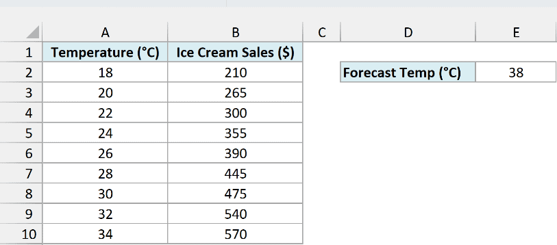
I want to estimate the sales for that 38-degree day using the fitted line.

Here is the formula:

=SUM(LINEST(B2:B10,A2:A10)*HSTACK(E2,1))

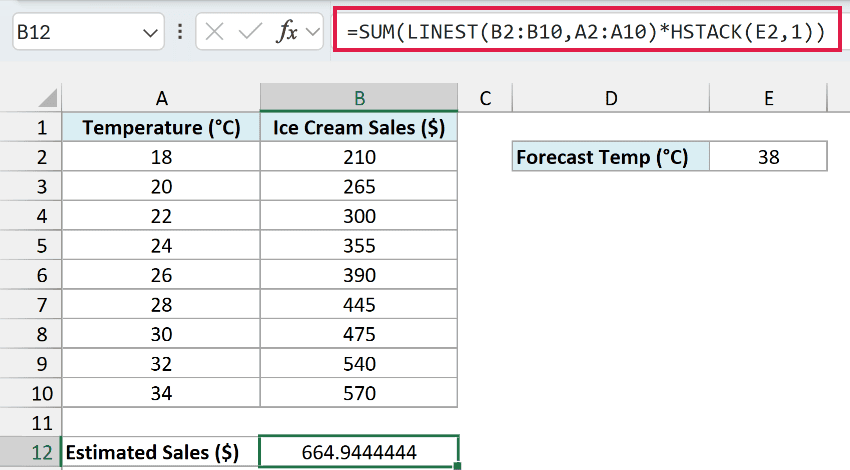
This returns about $665 in sales for a 38-degree day.

LINEST gives back {slope, intercept}, which is {22.5417, -191.6389} here. HSTACK(E2,1) builds {38, 1} to match it.

Multiplying pairs them up as slope × 38 and intercept × 1, and SUM adds the two pieces into the prediction.

Important: HSTACK works only in Excel for Microsoft 365 and Excel 2024. In older versions, use the TREND formula from the tip below.

Important: R-squared measures fit, not cause. And 38 degrees sits outside the 18 to 34 range in the data, so treat this as a rough estimate.

Pro Tip: For a plain prediction like this, the TREND function does it in one step: =TREND(B2:B10,A2:A10,E2). Use LINEST when you also want the coefficients.

Example 7: Skip Blank or Error Rows Before Fitting

Real data has gaps. Let’s fit a line while ignoring rows where a sensor didn’t report.

Below is a table of trail-counter days over fourteen days in A2:B15. Column A has the rainfall in millimeters, and column B has the hiker count.

A few rows have blanks or errors where the sensors failed.

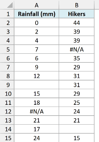
I want to keep only the days where both rainfall and hiker count are real numbers, then fit the line on those clean rows.

Here is the formula:

=LET(valid,ISNUMBER(A2:A15)*ISNUMBER(B2:B15),LINEST(FILTER(B2:B15,valid),FILTER(A2:A15,valid),TRUE,TRUE))

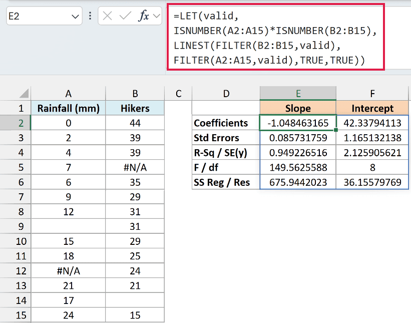
After filtering, ten days remain, and the line comes back with a slope of about -1.0485 and an intercept of 42.3379. R-squared is 0.9492.

So each extra millimeter of rain is linked to about one fewer hiker, starting from roughly 42 hikers on a dry day. Here is how the formula holds together:

• ISNUMBER(A2:A15)*ISNUMBER(B2:B15) builds a mask that is 1 only where both columns hold numbers.
• FILTER applies that same mask to each column, so the x and y values stay paired up and aligned.
• LINEST then fits the regression on the matched, clean arrays.

Important: Use one shared mask for both columns. Clean them separately and the rows can shift out of line, or LINEST returns #REF! when the sizes differ.

Important: LET and FILTER need Excel for Microsoft 365 or Excel 2021 and later. In older versions, clean the data first and run LINEST on the clean rows.

Example 8: Fit a Quadratic (Polynomial) Curve with LINEST

LINEST fits curves too, as long as you hand it the right predictors. Let’s fit a quadratic where a straight line won’t do.

Below is a table of electric-scooter braking tests. Column A has the speed in km/h, and column B has the braking distance in meters, over nine tests in A2:B10.

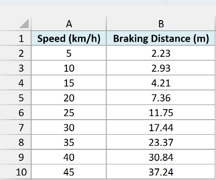
Braking distance grows faster than speed, so a straight line is a poor fit. I want to fit a curve using both speed and speed squared.

Here is the formula:

=LINEST(B2:B10,A2:A10^{1,2},TRUE,TRUE)

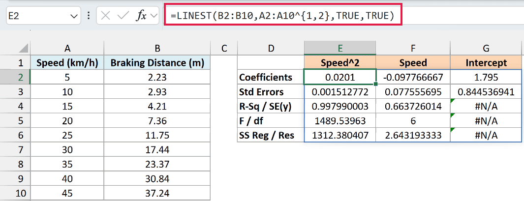
The A2:A10^{1,2} part raises the speed column to the first and second power, creating two predictor columns in memory.

LINEST then fits both at once and spills a 5-row by 3-column block.

Reading row 1 from left to right, and remembering the reverse order, you get:

• 0.0201 for speed squared (the x-squared term).
• -0.0978 for speed (the x term).
• 1.7950 for the intercept.

So the fitted curve is braking distance = 0.0201 × speed² – 0.0978 × speed + 1.7950. The squared term bends the line upward as speed climbs.

R-squared in row 3 is 0.9980, a tight fit.

LINEST gives you the full regression story in one formula: the slope and intercept, how well the line fits, and every stat behind it.

Start with a plain slope and intercept, add stats when you need them, and use INDEX or FILTER when you want one number or clean data first.

The two things to keep in mind are the output layout and the reversed coefficient order. Once those click, reading a LINEST result gets easy.

I hope you found this tutorial helpful.

List of All Excel Functions

Other Excel Articles You May Also Like:

• How to Add a TrendLine in Excel Charts (Step-by-Step Guide)
• How to Calculate Correlation Coefficient in Excel (2 Easy Ways)
• 20 Advanced Excel Functions and Formulas (for Excel Pros)
• How to Calculate Variance in Excel (Sample vs Population)