GROUPBY Function in Excel

If you want to summarize your data by category, you can do it with a single GROUPBY formula in Excel.

GROUPBY is a dynamic array function. You type it once and the whole summary table spills into the cells below and to the right.

It only works in Microsoft 365.

In this article, I’ll show you how to use GROUPBY in Excel to sum, average, count, group dates, and combine text.

Excel GROUPBY Function Syntax

Here is the syntax of the GROUPBY function:

=GROUPBY(row_fields,values,function,[field_headers],[total_depth],[sort_order],[filter_array],[field_relationship])

• row_fields is the column or columns you want to group by. These become the row labels. You can also supply calculated labels, as we’ll do with dates in Example 4.
• values is the column or columns you want to calculate something from, such as prices to add or names to count.
• function tells GROUPBY what calculation to run for each group. Write the function name on its own, like SUM, not SUM(). Other choices include AVERAGE, COUNT, MEDIAN, MIN, MAX, PERCENTOF, and ARRAYTOTEXT.
• field_headers is optional. Use 0 when the ranges have no headers, 1 when they have headers but you want to hide them, 2 when they have no headers but you want generated ones, or 3 to show the source headers. Omit it for automatic detection.
• total_depth is optional. Omit it for automatic totals, including subtotals where possible. Use 0 for no totals, 1 for a grand total, or 2 for a grand total and subtotals. Use -1 or -2 for the same totals at the top. Subtotals need at least two grouping columns.
• sort_order is optional. It points at an output column, counting the grouping columns first, then the value columns. A positive number sorts ascending; a negative number sorts descending. By default, GROUPBY sorts the row labels A to Z.
• filter_array is optional. It’s a column of TRUE/FALSE results, one per source row. GROUPBY includes TRUE rows before grouping. It must have the same number of rows as row_fields.
• field_relationship is optional and only matters with multiple grouping columns. Use 0 (the default) for a hierarchy, with later columns grouped inside earlier ones. Use 1 for table mode, where columns sort independently and subtotals aren’t available.

The first three arguments are all you need for most summaries. The other five are switches you turn on when you want more control.

GROUPBY is available in Excel for Microsoft 365. Excel 2024, Excel 2021, and older perpetual versions don’t include it and show #NAME? for a GROUPBY formula.

For an alternative to GROUPBY in Excel, use a PivotTable.

In Excel 2021 or later, you can also combine UNIQUE with SUMIFS for a total per group.

When to Use the GROUPBY Function

Use GROUPBY when you need to:

• Build a summary grouped by a category, all from one formula.
• Get sums, averages, counts, or text lists per group without a PivotTable.
• Group dates by month or year without adding a helper column.
• Create a summary with multiple grouping levels and subtotals.
• Keep a summary that recalculates when the source data changes.

Let me show you a few practical examples of how this works.

Example 1: Group and Sum Data by Category

Let’s start with a simple example.

Below is a list of ten grocery items and their prices, and I want total spend for each aisle in columns E and F.

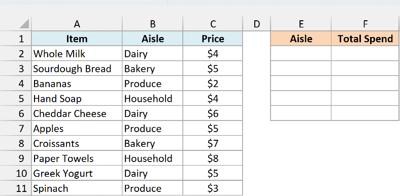
Here is the formula:

=GROUPBY(B2:B11,C2:C11,SUM)

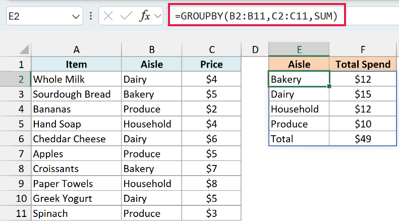
Here, the first argument (B2:B11) is the Aisle column I want to group by. The second argument (C2:C11) is the Price column I want to add up.

And SUM tells GROUPBY to total each group.

The result spills into E2:F6. Each aisle shows up once with its total next to it: Bakery $12, Dairy $15, Household $12, and Produce $10.

The aisles come out sorted A to Z automatically. You also get a Total row at the bottom that adds up to $49.

GROUPBY adds that Total row by default. Set total_depth to 0 to remove it, as you’ll see in Example 6.

Notice that I did not touch the Item column at all. GROUPBY only cares about the columns you hand it.

If row_fields and values cover different numbers of rows, GROUPBY returns #VALUE! because each grouping label needs a matching value.

When you use filter_array, it must cover the same number of rows too, so the filter lines up with the source data.

Anything already in E2:F6 blocks the result and causes a #SPILL! error, so keep that area empty before entering the formula.

Pro Tip: Use Excel Table column references to include new rows automatically. Keep the GROUPBY formula outside the Table, as it can’t spill inside one.

Example 2: Average per Group with Source Headers

Here’s another practical scenario.

Below are 12 test scores, and I want the average score for each subject, with the source headers included, in columns E and F.

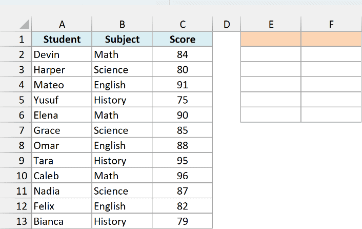
Here is the formula:

=GROUPBY(B1:B13,C1:C13,AVERAGE,3)

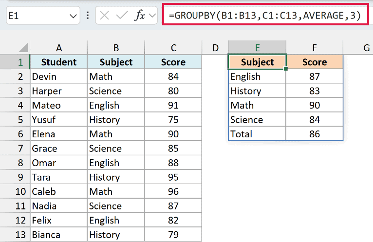
This time, the ranges start at row 1, so they include the Subject and Score headers. AVERAGE tells GROUPBY to average the scores in each subject.

The 3 is field_headers. It tells GROUPBY that the source ranges have headers and that those headers should appear in the result.

E1:F1 shows Subject and Score. Below that come English 87, History 83, Math 90, and Science 84, followed by Total 86.

When field_headers is omitted, GROUPBY checks the values argument to decide whether the first row contains headers.

If its first value is text and the second is a number, GROUPBY treats that first row as headers.

In this dataset, it would recognize the headers but hide them. Setting field_headers to 3 makes them appear in the result.

When the headers matter, set field_headers yourself instead of relying on auto-detection.

The Total row averages all 12 original scores: 1032 divided by 12 gives 86.

It equals the average of the four subject averages here because each subject has three scores. With uneven group sizes, those two averages can differ.

Example 3: Count Items in Each Group

Now let’s look at something a little different.

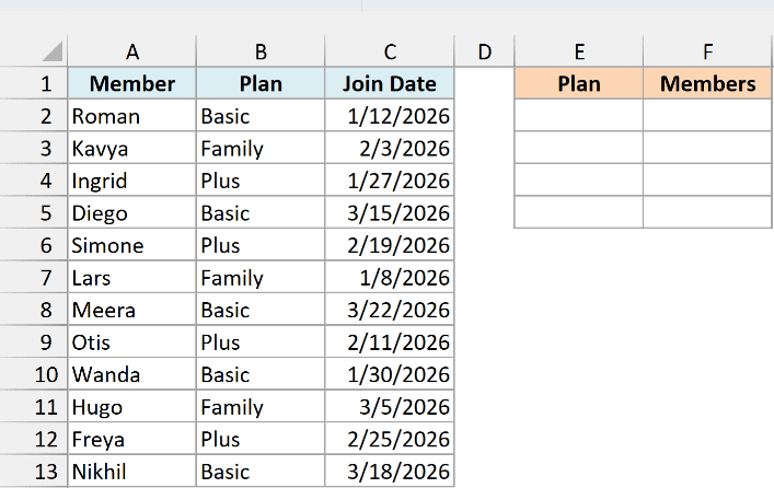
I have a list of 12 gym members, and I want to count how many are on each plan in columns E and F.

Here is the formula:

=GROUPBY(B2:B13,A2:A13,COUNTA)

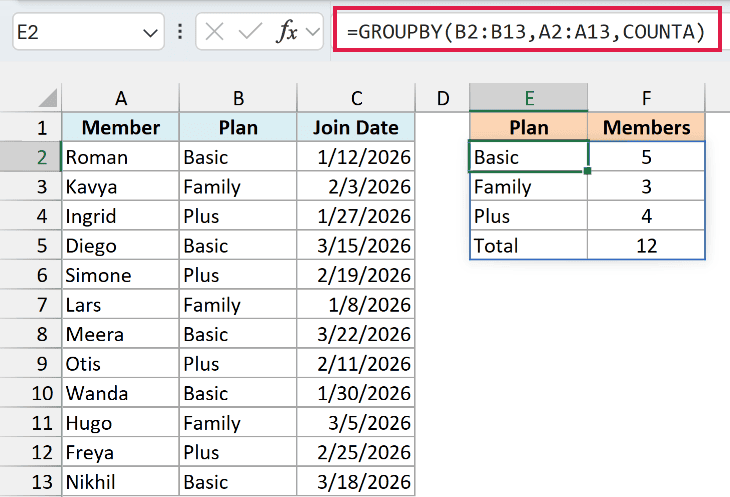
This time I grouped by the Plan column (B2:B13) and pointed the values at the Member column (A2:A13). COUNTA counts the names in each group.

The result in E2:F5 shows Basic 5, Family 3, and Plus 4, with a Total of 12.

There is a reason I used COUNTA here and not COUNT. COUNTA counts non-empty cells, including names.

COUNT only counts numbers, so pointing it at this column of names would return 0 for every group.

Example 4: Group Dates by Month with GROUPBY

Let’s group dates next, without adding a helper column.

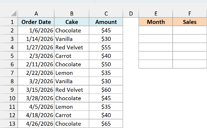
Below are 12 cake orders from a home bakery, and I want total cake sales for each month in columns E and F.

Here is the formula:

=GROUPBY(TEXT(A2:A13,"yyyy-mm"),C2:C13,SUM)

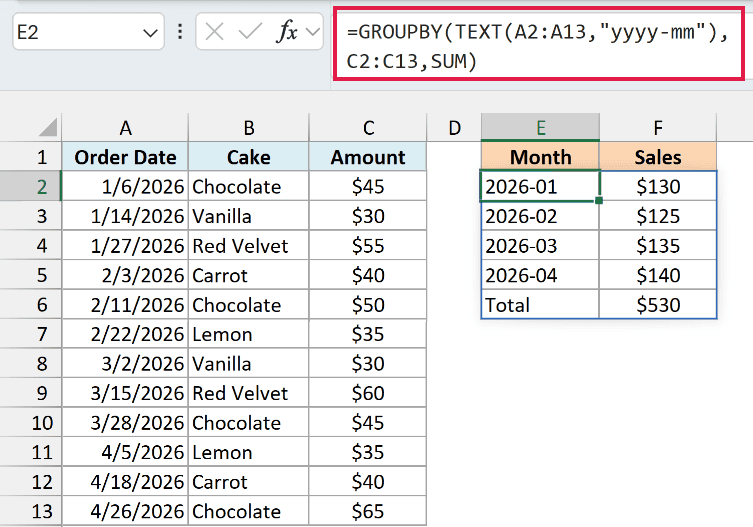
The result in E2:F6 shows 2026-01 $130, 2026-02 $125, 2026-03 $135, and 2026-04 $140. The Total row is $530.

Here is how this formula works:

• TEXT converts each date in A2:A13 into a year-month label using "yyyy-mm".
• GROUPBY uses those calculated labels as row_fields. This argument doesn’t have to be a range of cells already on the sheet.
• C2:C13 supplies the order amounts, and SUM adds them for each month.

If you want totals by year instead of month, use TEXT(A2:A13,"yyyy") as the first argument.

The month labels from the TEXT function are text. If you need real dates for date math, use DATE(YEAR(A2:A13),MONTH(A2:A13),1) as row_fields instead.

Then format E2:E5 with the custom number format mmm yyyy to show those dates as labels like Jan 2026.

Important: With “mmm” labels, GROUPBY sorts A to Z: Apr, Feb, Jan, Mar. Use “yyyy-mm” to keep months in date order and different years apart.

Example 5: GROUPBY with Multiple Columns and Subtotals

Let’s step it up with two grouping levels.

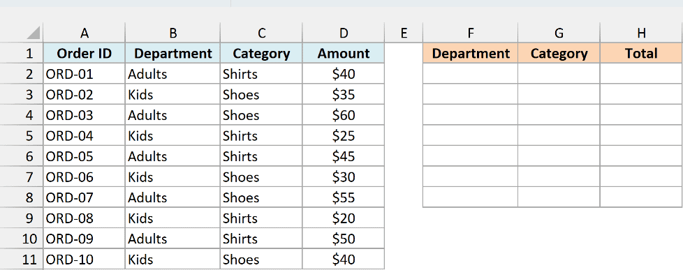
I have ten clothing store orders, and I want totals by department and category, with department subtotals, in columns F, G, and H.

Here is the formula:

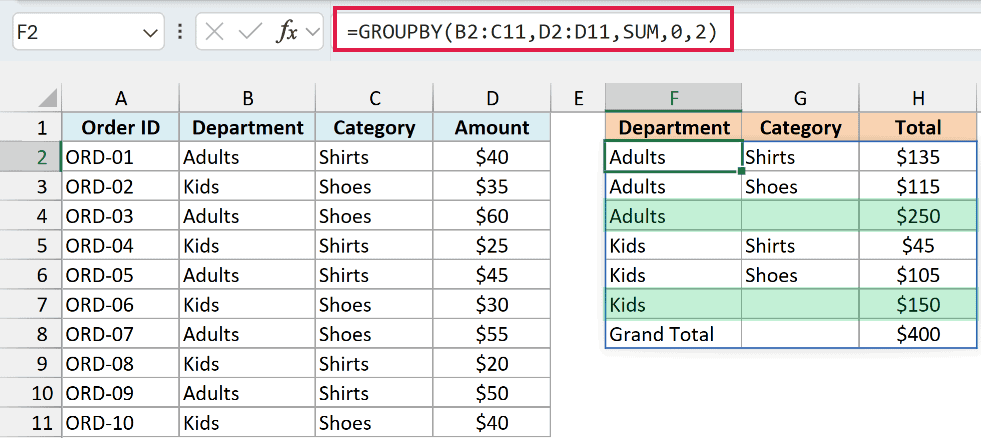
=GROUPBY(B2:C11,D2:D11,SUM,0,2)

Here is how this formula works:

• B2:C11 covers two grouping columns. GROUPBY groups by Department first, then by Category inside each department.
• D2:D11 supplies the order amounts, and SUM adds them for each Department and Category combination.
• 0 is field_headers. The selected source ranges start at row 2, so they don’t include a header row.
• 2 is total_depth. It asks for department subtotals and a grand total.

The Adults rows show Shirts $135 and Shoes $115, followed by an Adults subtotal of $250.

The Kids rows show Shirts $45 and Shoes $105, followed by a Kids subtotal of $150. The last row is Grand Total $400.

Each subtotal sits immediately after that department’s category rows. It repeats the department name and leaves Category blank.

The Grand Total row also leaves Category blank.

If you want the largest category amounts first, set sort_order to -3, because the amount is output column 3.

This sorts categories by amount, largest first, within each department. Departments stay in A to Z order.

Subtotals need at least two grouping columns. Setting total_depth to 2 with only one grouping column returns #VALUE!.

If your grouping columns aren’t next to each other, combine them with the HSTACK function or select them with the CHOOSECOLS function for the row_fields argument.

Example 6: Filter and Sort the GROUPBY Summary

This next one uses two of the optional arguments together.

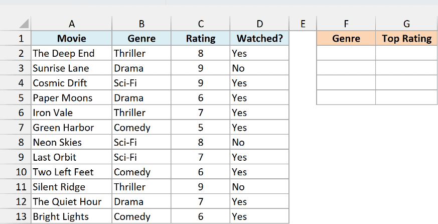
Below is a watchlist of 12 movies, and I want the highest rating per genre for movies marked Yes under Watched?, sorted highest first, in columns F and G.

Here is the formula:

=GROUPBY(B2:B13,C2:C13,MAX,0,0,-2,D2:D13="Yes")

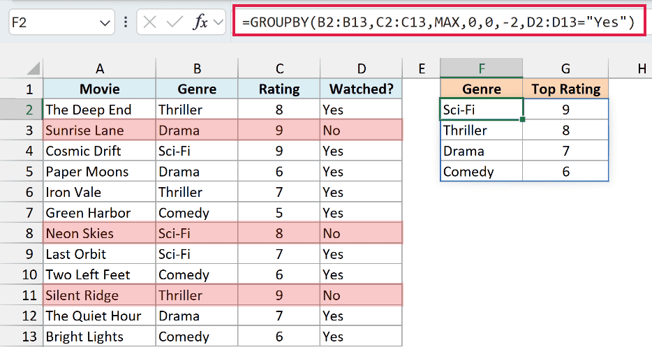
The result in F2:G5 gives Sci-Fi 9 at the top, then Thriller 8, Drama 7, and Comedy 6. The movies marked No never enter the calculation.

Here is how this formula works:

• B2:B13 supplies the genres, and C2:C13 supplies the ratings. MAX returns the highest included rating in each genre.
• The first 0 sets field_headers, because the selected ranges don’t include headers.
• The second 0 sets total_depth, turning off the Total row. A grand maximum across genres isn’t needed for this list.
• -2 sets sort_order to the second output column, the rating, from largest to smallest. Count output positions, not source columns.
• D2:D13="Yes" is filter_array. It returns TRUE for watched movies and FALSE for the rest, so only watched rows reach GROUPBY.

Silent Ridge (Thriller 9) and Sunrise Lane (Drama 9) are both unwatched. Without the filter, Thriller and Drama would each show 9.

The filter_array screens source rows before grouping. It can’t hide groups based on their finished totals.

To filter the finished summary instead, wrap the result in FILTER.

Example 7: Run Several Calculations at Once

Now let’s get more than one calculation for each group.

Below are 12 household bills, and I want the total, average, and share of all spending for each bill type in columns E, F, G, and H.

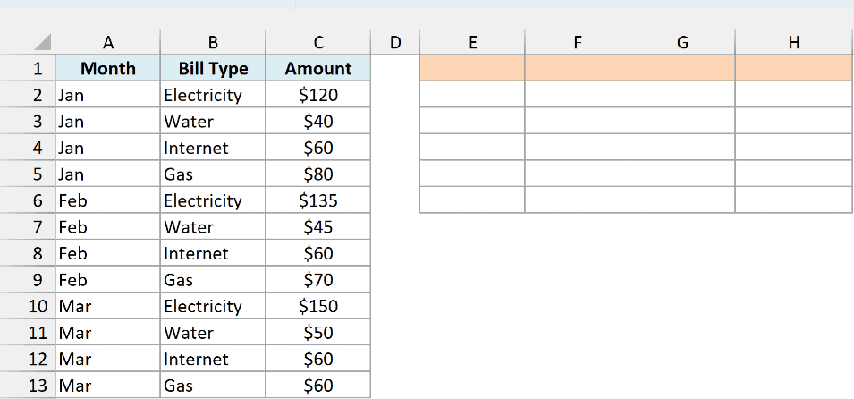
Here is the formula:

=GROUPBY(B2:B13,C2:C13,HSTACK(SUM,AVERAGE,PERCENTOF),0)

Here is how this formula works:

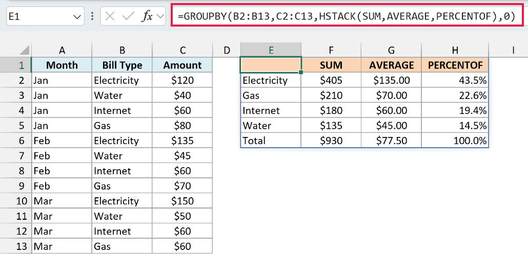
• B2:B13 groups the bills by Bill Type, and C2:C13 supplies the amounts. The Month column isn’t used.
• HSTACK(SUM,AVERAGE,PERCENTOF) supplies three functions side by side. GROUPBY runs all three for each bill type.
• SUM gives each bill type’s total. AVERAGE gives its average bill, and PERCENTOF gives its share of the grand total.
• 0 is field_headers, because the selected source ranges don’t include headers.

GROUPBY labels F1:H1 as SUM, AVERAGE, and PERCENTOF, in capitals. E1 is blank. These are calculation labels created by the formula.

GROUPBY adds this label row whenever you supply several functions, regardless of field_headers, so the 0 doesn’t create it.

Electricity shows $405, $135.00, and 43.5%. Gas shows $210, $70.00, and 22.6%.

Internet shows $180, $60.00, and 19.4%. Water shows $135, $45.00, and 14.5%.

The Total row shows $930, $77.50, and 100.0%. Its AVERAGE is the average of all 12 original bills.

You can pass several functions to GROUPBY with the HSTACK function for calculations across columns, as in this example.

To put the calculations down rows instead, use the VSTACK function. It stacks them as extra rows under each group.

If you need a calculation of your own, GROUPBY also accepts a custom LAMBDA function, as I’ll show in Example 8.

Pro Tip: GROUPBY returns plain numbers. Format F2:F6 as currency, G2:G6 as currency with two decimals, and H2:H6 as percentages. Formatting stays when the data updates.

Example 8: Combine Text by Group

Let’s finish by grouping names into text lists.

I have 12 party RSVPs, and I want one comma-separated list of guest names for each answer in columns D and E.

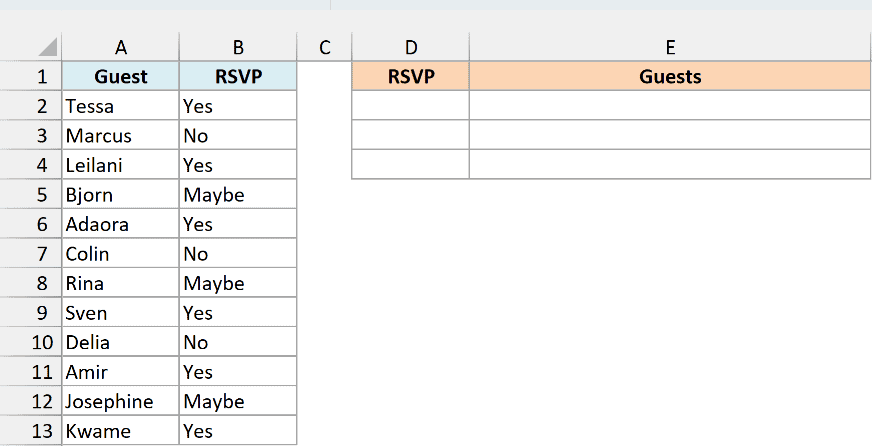
Here is the formula:

=GROUPBY(B2:B13,A2:A13,ARRAYTOTEXT,0,0)

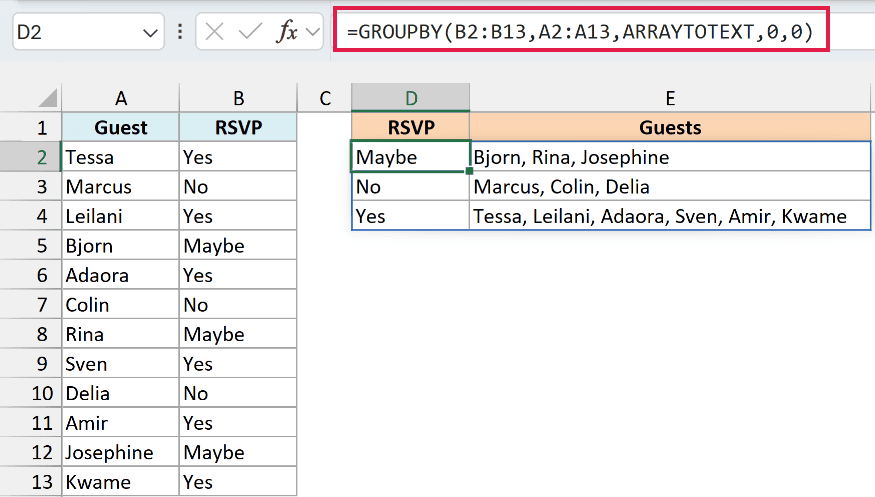
GROUPBY isn’t only for numbers. Here it groups by RSVP in B2:B13 and passes each group’s names from A2:A13 to ARRAYTOTEXT.

ARRAYTOTEXT joins the names with a comma and a space, keeping them in source order within each group.

Maybe gives “Bjorn, Rina, Josephine”, and No gives “Marcus, Colin, Delia”.

Yes gives “Tessa, Leilani, Adaora, Sven, Amir, Kwame”. These three rows fill D2:E4.

The two zeros set field_headers and total_depth to 0. There are no formula-generated headers and no Total row combining all the names.

For a different separator, pass your own LAMBDA as the function argument.

For example, use =GROUPBY(B2:B13,A2:A13,LAMBDA(x,TEXTJOIN(" | ",TRUE,x)),0,0) for names separated by | .

The LAMBDA receives each group’s names as x, and TEXTJOIN joins them using that separator.

In this article, I showed you how to use GROUPBY to sum, average, count, group dates by month, and add subtotals.

I also covered filtering and sorting, running several calculations at once, and combining text by group.

The PIVOTBY function is GROUPBY’s sibling. Use it when you also want groups spread across columns.

I hope you found this article helpful.

List of All Excel Functions

Other Excel Articles You May Also Like:

• Group Dates in Pivot Tables in Excel
• Combine Duplicate Rows and Sum the Values in Excel
• COUNTIF Function in Excel
• Table.Group Function in Power Query M
• SUBTOTAL Function in Excel