

The SQRTPI function in Excel multiplies a number by pi, then returns the square root of that product. Pi is the mathematical constant approximately equal to 3.14159.
It’s useful when a calculation has pi inside a square root, including finding a circle’s circumference when you know its area. A whole range needs a small adjustment before SQRTPI can calculate each value, which I’ll show you below.
Follow along with the example file
SQRTPI Function Examples.xlsx
SQRTPI Function Syntax
Here is the syntax of the SQRTPI function:
=SQRTPI(number)
- number (required): The value to multiply by pi before taking the square root. You can supply a number, a cell reference, or a calculation that returns a number.
The input can be zero or a positive number, including a decimal. You don’t supply pi as a separate argument because SQRTPI already includes it in the calculation.
SQRTPI works in Excel for Microsoft 365, Excel 2024, 2021, 2019, and 2016. The spilling examples below need Microsoft 365, Excel 2024, or Excel 2021; older-version formulas are included beside them.
When to Use the SQRTPI Function
Use SQRTPI when you need to:
- Calculate the square root of a number multiplied by pi.
- Apply that calculation to a list of numeric inputs.
- Find the distance around a circle from its area, without calculating the radius in a separate cell.
Let’s work through these examples, then look at the inputs that can cause errors.
Example 1: Calculate a Single SQRTPI Result
Let’s start with one number so you can see the order of the calculation.
Below is the number 3 in cell B1, and I want the square root of its product with pi in cell B3.
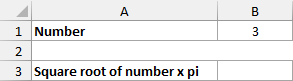
On the Example 1 sheet, enter this formula in cell B3:
=SQRTPI(B1)
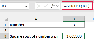
The formula returns 3.069980, as displayed to six decimal places in the workbook. It first multiplies 3 by pi to get approximately 9.424778, then takes the square root of that product.
The whole product is inside the square root. Taking the square root of 3 first and multiplying that answer by pi would give a different result.
Here we’re using a single cell to make that calculation easy to follow. The next example applies it to several numbers at once.
Example 2: Calculate a List of Results
A list introduces one extra detail with SQRTPI.
Below are eight numbers, including zero and fractions, and I want their SQRTPI results in column B.
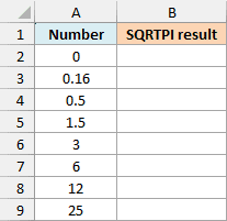
On the Example 2 sheet, enter this formula in cell B2 and press Enter:
=SQRTPI(+A2:A9)
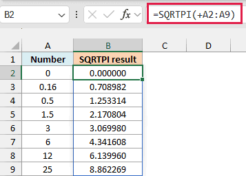
The formula fills B2:B9 automatically, with one answer for each input. This is called spilling, so you only enter the formula once.
For example, 0 returns 0.000000, 0.16 returns 0.708982, and 25 returns 8.862269. The results use six decimal places for display; Excel keeps the underlying precision for later calculations.
The plus sign before A2:A9 makes Excel evaluate the range as an array of values before passing it to SQRTPI. It doesn’t add anything to the numbers.
Important: Passing the bare range as =SQRTPI(A2:A9) returns #VALUE!. Keep the leading + in this numeric-list formula so SQRTPI receives the values in a form it can process.
This is one of the Excel functions that need an adjustment to spill. The example contains numbers only; the last example checks direct references to other input types separately.
If the output cells contain something already, Excel returns #SPILL!. Move or remove the entries blocking B2:B9, then enter the formula in B2 again.
If you’re using Excel 2019 or earlier, enter the below formula in cell B2 and copy it down through B9:
=SQRTPI(A2)
Example 3: Find Circular Garden Edging Length
Now let’s use SQRTPI in a calculation with a practical result.
Below are six circular flower beds with their areas in square meters, and I want the length of edging around each bed in column C.
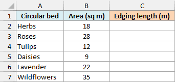
On the Example 3 sheet, enter this formula in cell C2:
=2*SQRTPI(+B2:B7)
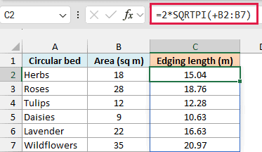
The formula returns 15.04 meters for the Herbs bed, which has an area of 18 square meters. All six answers spill into column C, with two decimal places shown in the workbook.
A circle’s area is pi multiplied by its radius squared, while its circumference is twice pi multiplied by its radius. Combining those relationships gives circumference as twice the square root of pi multiplied by area.
SQRTPI calculates the square-root part using each area in B2:B7. Multiplying by 2 gives the circumference, which is the distance around the bed.
As in the previous example, the leading plus sign lets SQRTPI work with the numeric range. Because the areas are in square meters, taking the square root gives a length in meters.
Important: This calculation assumes each bed is circular. The result is its geometric circumference, so it doesn’t include extra material for cutting, joins, or overlap.
If you’re using Excel 2019 or earlier, enter the below formula in cell C2 and copy it down through C7:
=2*SQRTPI(B2)
Example 4: Check Inputs That Cause Errors
An unexpected result can come from the input itself.
Below are several input types, and I want to see how SQRTPI handles each one in column C.
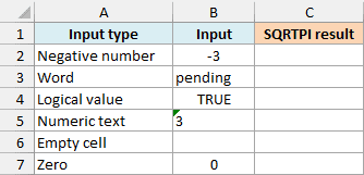
On the Example 4 sheet, enter this formula in cell C2 and copy it down through C7:
=SQRTPI(B2)
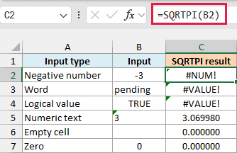
Here we use separate formulas because we’re testing direct references to individual cells. Adding an arithmetic operator to make an array can change how some input types are treated, which would make this a different test.
The negative input, -3, returns #NUM! because its product with pi has no real square root. Check whether a negative value belongs in your calculation before changing it to a positive number.
The word pending and the logical value TRUE both return #VALUE!. Neither is an accepted numeric input in this direct-reference example, so replace it with the intended number once that number is known.
The numeric text in B5 is the digit 3 stored as text, and SQRTPI accepts it. It returns 3.069980, the same answer as the number 3 in Example 1.
Both the genuinely empty input cell and the zero input return 0.000000. An empty cell therefore doesn’t leave the answer empty.
Important: A zero result can mean the referenced input is empty. If an empty cell means a measurement is missing, fill in that measurement before treating the result as a valid zero.
These examples show how SQRTPI handles a single number, a numeric list, and a calculation using circle areas. The input checks also help explain why an error or an unexpected zero appears.
Other Excel Articles You May Also Like:
