
Today I am going to give you a powerful formula cocktail. The less-used INDIRECT() and ROW() function together with the MID() function can create a magnificent concoction.
This triad enables you to get into the contents in a cell. and analyze each character separately. For example, suppose you have Excel123 in a cell, and you want to identify if it contains a numeric value or not (which it does!!). Excel inbuilt formulas can not help you here as excel consider this as text (Try and use Type() function to see for yourself).
What you need here is a way to check each character separately and then identify if it contains a number. Lets first have a look at the formula that can separate each character:
=MID(B2,ROW(INDIRECT("1:"&LEN(B2))),1)
Here this works:
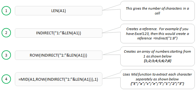
Now when you have it all dissected, you are free to analyze each character separately.
Note that this technique is best used when combined with other formulas (as you will see later in this post). As a stand-alone technique, it could hardly be of any use. Also, Indirect() is a volatile function, so use cautiously. [Know more about volatile formula]
Here are a few examples where this technique could be helpful:
1. To identify cells that contain a numeric character:
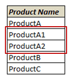
Suppose you have a list as shown below, and you want to identify (or filter) any cell that contains a numeric character anywhere in the cell
 To do this, use the following formula. It returns a True if a cell contains any numeric character, and False if it doesn’t.
=OR(ISNUMBER(MID(A2,ROW(INDIRECT(“1:”&LEN(A2))),1)*1))
Use Control + Shift + Enter to enter this formula (instead of Enter), as it is an array formula.
2. To identify the position of the first occurrence of a number
To do this, use the following formula. It returns the position of the first occurrence of a number in a cell. For example, if a cell contains ProductA1, it will return 9. In case there is no number, it returns “No Numeric Character Present”
=IFERROR(MATCH(1,–ISNUMBER(MID(B3,ROW(INDIRECT(“1:”&LEN(B3))),1)*1),0),”No Numeric Character Present”)
Use Control + Shift + Enter to enter this formula
Hope this saves you some time and effort. If you come up with any other way to use this technique, do share it with me as well.


