AREAS Function in Excel

The AREAS function in Excel tells you how many areas a reference contains. An area is a single cell or a block of cells next to each other, so B2:D9 is one area, while B2:B9 and D2:D9 together make two.

You’ll mostly use it to check how many blocks a named range or print area covers, or to get a block number for the INDEX function. In this tutorial, I’ll show you how all of that works with seven examples.

AREAS Function Syntax

Here is the syntax of the AREAS function:

=AREAS(reference)

• reference – the cell, range, or named range whose areas you want to count. It can also be several ranges combined into one reference.

To give AREAS more than one range, separate the ranges with commas and wrap the whole list in an extra pair of parentheses, like =AREAS((B2:B9,D2:D9)). The inner parentheses turn the list into one reference, so AREAS still gets a single argument.

The argument has to be a real reference. If you type a value instead, such as =AREAS("B2:D9") or =AREAS(5), Excel won’t accept the formula, because there are no cells for AREAS to count.

The AREAS function works in Excel 365, 2024, 2021, 2019, 2016, and Excel for Mac.

When to Use the AREAS Function

Use this function when you need to:

• Check how many separate blocks a named range covers.
• Count the print areas set on a sheet before you print it.
• Find out whether two ranges overlap.
• Get the number of the last block in a range, so the INDEX function can return it.
• Work through every block of a multi-area range in one formula.

Let me show you a few practical examples of how to use the AREAS function.

Example 1: Count the Areas in a Range

Let’s start with a simple example.

Below is a table of monthly household bills, and I want to count the areas in two different references in column G.

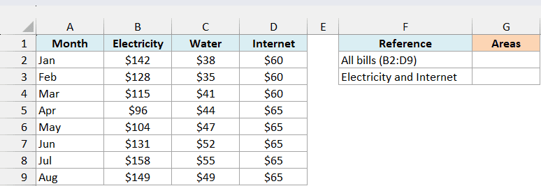
Here is the formula for the whole table of bills:

=AREAS(B2:D9)

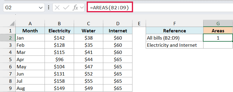
This returns 1. B2:D9 covers 24 cells, but it’s one rectangular block of cells, so it counts as one area.

Now let’s count the Electricity and Internet columns together. Here is the formula in G3:

=AREAS((B2:B9,D2:D9))

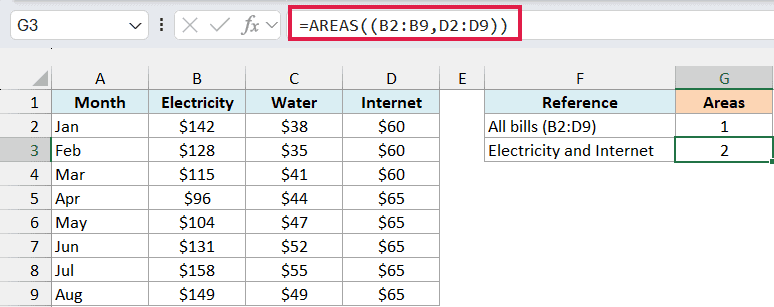
This returns 2. The comma joins the two ranges into one reference (Excel calls this the union operator), and AREAS counts each range you join this way as its own area.

As you’ll see in the next example, that’s true even when the joined ranges sit right next to each other.

Important: Don’t drop the extra pair of parentheses. If you type =AREAS(B2:B9,D2:D9), Excel reads the comma as the start of a second argument and won’t accept the formula.

All the ranges in a union also have to be on the same sheet. A reference such as (B2:B9,'Example 2'!B2:B8) makes AREAS return #VALUE!.

Example 2: Adjacent and Overlapping Ranges Count Separately

Now let’s see what AREAS does when the ranges touch or overlap.

Below is a step counter log for two weeks, and I want to count the areas in two references in column F.

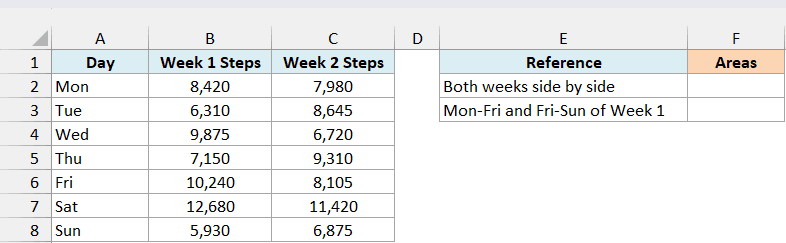
Here is the formula for the two week columns:

=AREAS((B2:B8,C2:C8))

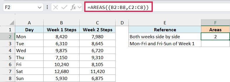
This returns 2, even though B2:B8 and C2:C8 sit right next to each other. AREAS counts the pieces you put in the reference, not the shape they make on the sheet.

Next, here is a formula where the two ranges share cell B6 (Friday of Week 1):

=AREAS((B2:B6,B6:B8))

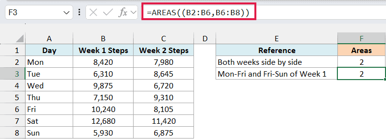
This also returns 2. Excel doesn’t merge overlapping pieces, so B6 belongs to both areas.

Important: If you add up an overlapping union, the shared cells are counted twice. =SUM((B2:B6,B6:B8)) returns 70,845 instead of 60,605, because Friday’s 10,240 steps are added twice, so use one continuous range like B2:B8 for a total.

Example 3: Count the Areas in a Named Range

AREAS also works with named ranges, and this is where it starts to get useful.

Below is a party budget where the named range BudgetInputs covers only the cells you type amounts into, and I want to check how many blocks it has in F2.

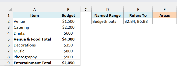
Here is the formula:

=AREAS(BudgetInputs)

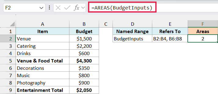
This returns 2. The Venue & Food Total in B5 is a subtotal, not an input, so the name skips it, and that splits the input cells into two blocks (B2:B4 and B6:B8).

This makes AREAS a quick check on any named range. If the count is higher than you expected, the name may include an extra cell, skip one in the middle, or be built from touching pieces that still count separately (as in Example 2).

Pro Tip: To see exactly which cells a name covers, pick it from the Name Box (to the left of the formula bar). Excel selects every area of the name at once, so the gaps are easy to spot.

Example 4: Count the Print Areas on a Sheet

Excel lets you set more than one print area on a sheet, and each one prints on its own page. When you set a print area, Excel saves it as a named range called Print_Area for that sheet, so AREAS can count them.

Below is a sheet with two small reports, a product list and monthly revenue, both set as print areas (A1:B7 and D1:E7), and I want to count the print areas in I2.

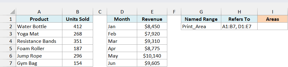
Here is the formula:

=AREAS(Print_Area)

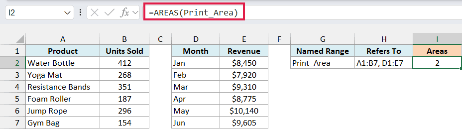
This returns 2, so this sheet prints as two pages.

Every sheet that has a print area gets its own Print_Area name. So to check a different sheet, include the sheet name, like =AREAS('Example 4'!Print_Area), because the plain name returns #NAME? on a sheet without a print area.

Example 5: Check Whether Two Ranges Overlap

AREAS can also tell you whether two ranges share any cells.

Below is a gym’s weekly class attendance, and I want to check two pairs of ranges for overlap in column I.

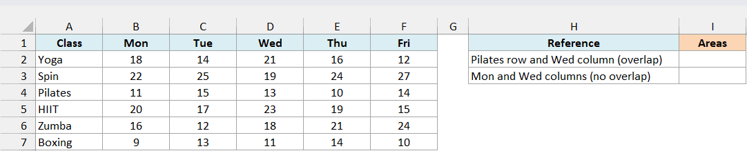
Here is the formula that checks the Pilates row against the Wednesday column:

=AREAS(B4:F4 D2:D7)

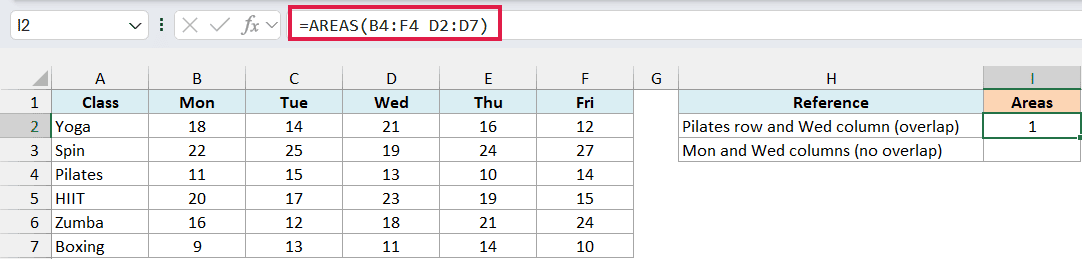
This returns 1. The space between the two ranges is the intersection operator, which returns only the cells both ranges share.

Here the shared cell is D4 (Pilates on Wednesday), so there’s one area.

Now here is the formula for two ranges that don’t touch, the Monday and Wednesday columns:

=AREAS(B2:B7 D2:D7)

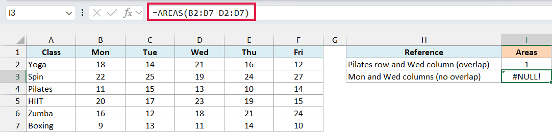
This returns #NULL!. The two columns have no cells in common, so the intersection is empty and there’s nothing for AREAS to count.

So a number means the ranges overlap, and #NULL! means they don’t.

Example 6: Get the Last Area With INDEX and AREAS

Let’s step it up and use AREAS inside another formula.

Below are monthly expenses where the named range MonthlyExpenses holds each month’s column as its own area, and I want the total for the latest month in H2.

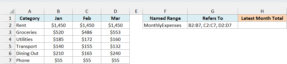
Here is the formula:

=SUM(INDEX(MonthlyExpenses,0,0,AREAS(MonthlyExpenses)))

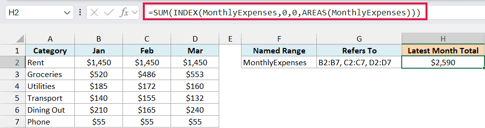
How this formula works:

• AREAS(MonthlyExpenses) returns 3, the number of areas in the name.
• INDEX(MonthlyExpenses,0,0,3) uses the reference form of the INDEX function. A 0 for the row and the column means the whole area, and the last argument (area_num) picks the third area, D2:D7.
• SUM adds up that area, which gives $2,590 for March.

When April comes along, open Formulas > Name Manager and add April’s column to the end of what MonthlyExpenses refers to, as a separate area (for example, ,E2:E7). The formula then returns April’s total without any change to the formula itself.

The order matters here, because INDEX numbers the areas in the order they appear in the name. If you stretch D2:D7 to D2:E7 instead, AREAS still returns 3, and the formula quietly adds March and April together.

If the area number is bigger than the number of areas in the name, INDEX returns #REF!. Getting that number from AREAS means the formula can never point past the last area.

Example 7: Get a Total for Every Area in One Formula

Finally, let’s get a separate total for every area at once.

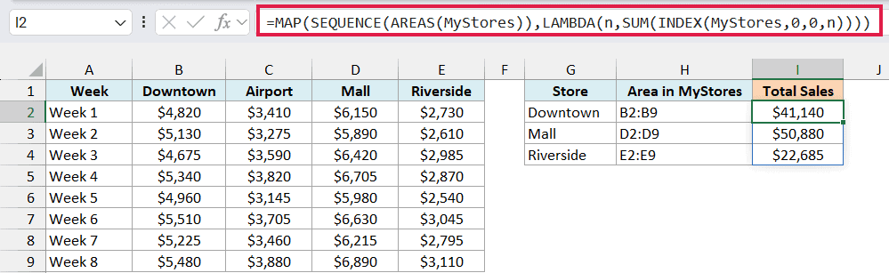
Below is weekly sales for four stores, where the named range MyStores covers three of them (Downtown, Mall, and Riverside), and I want a total for each of these stores in column I.

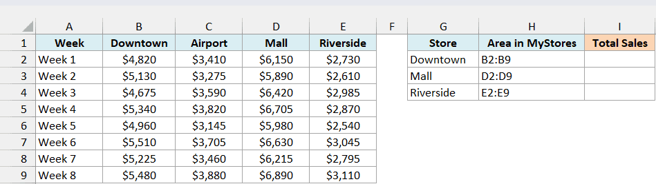
Here is the formula:

=MAP(SEQUENCE(AREAS(MyStores)),LAMBDA(n,SUM(INDEX(MyStores,0,0,n))))

How this formula works:

• AREAS(MyStores) returns 3, one for each store column in the name.
• SEQUENCE(3) creates the list 1, 2, 3.
• The MAP function passes each of those numbers to the LAMBDA as n, and SUM(INDEX(MyStores,0,0,n)) adds up area n.
• The three totals spill into I2:I4, in the same order as the areas in the name.

You might expect =SUM(INDEX(MyStores,0,0,SEQUENCE(3))) to at least add up all three areas (114,705). It returns 13,700 instead, which is just the first cell of each area added together.

MAP fixes this by handing INDEX one area number at a time, so each INDEX returns a whole area for SUM to add up.

The same INDEX trick helps with functions like ROWS, COLUMNS, and SUMIF, which don’t accept a multi-area reference at all (they return #REF! or #VALUE!). Pull out one area first with INDEX(MyStores,0,0,n), and then use the function on that area.

The MAP and LAMBDA functions need Excel 365 or Excel 2024. If you are using an older version, enter the below formula in cell I2 and then copy it down to I4:

=SUM(INDEX(MyStores,0,0,ROWS($I$2:I2)))

Here, ROWS($I$2:I2) counts the rows from I2 down to the current cell, so it gives 1 in I2, 2 in I3, and 3 in I4, and each row picks up the next area.

So that’s how the AREAS function works. It counts the blocks in a reference, and that count is most useful when you check a named range or a print area, or when you pass it to INDEX to reach a specific block.

List of All Excel Functions

Other Excel Articles You May Also Like:

• ROWS Function in Excel
• COLUMNS Function in Excel
• SHEETS Function in Excel
• COUNT Function in Excel
• OFFSET Function in Excel