

If you want to find out how many columns are in a range or an array, the COLUMNS function is the quickest way to do it. It takes a range and hands you back a single number, the count of columns in that range.
It’s a small function, but it does a lot of useful work inside bigger formulas. In this article, I’ll show you how COLUMNS works and five practical ways to put it to use.
COLUMNS returns a single number, but it works nicely inside dynamic array formulas. For example, =COLUMNS(A2#) counts the columns in a spilled range.
Follow along with the example file
COLUMNS Function Examples.xlsx
COLUMNS Syntax
Here is the syntax of the COLUMNS function:
=COLUMNS(array)
- array – the range, array, or array formula whose columns you want to count. This is the only argument, and it’s required.
The function looks only at the width of what you give it. The number of rows makes no difference, so COLUMNS(A1:D1) and COLUMNS(A1:D100) both return 4.
When to Use the COLUMNS Function in Excel
Use the COLUMNS function when you need to:
- Check how many columns wide a range or table is
- Feed a column index into a lookup formula so it updates as you copy it across
- Number columns in a row automatically
- Measure the width of a dynamic array that spills
One quick point before we start. COLUMNS (with an S) counts columns and returns how many there are. The COLUMN function (no S) returns the column number of a single cell, so COLUMN(C1) returns 3. This article is about COLUMNS, the counting one.
Let me show you a few practical examples of how to use this function.
Example 1: Count the Number of Columns in a Range
Let’s start with a simple example.
Below is a small product table with five columns: Product, Category, Stock, Price, and Supplier.
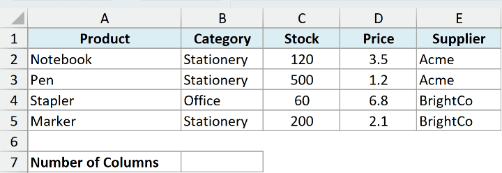
I want to know how many columns this table spans without counting them by hand.
Here is the formula:
=COLUMNS(A1:E1)
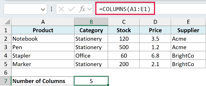
The range A1:E1 covers columns A through E, so COLUMNS returns 5.
You could also point it at the full data block like =COLUMNS(A1:E20) and still get 5. The rows never change the answer, only the number of columns does.
Pro Tip: If your data is in a named Excel Table, you can pass the table name straight in, like =COLUMNS(SalesData), and the count updates on its own when you add or remove columns.
Example 2: Build a Dynamic Column Index for VLOOKUP
Here’s a scenario I run into a lot.
Below is a table with a product in column A and its quarterly sales in columns B to E (Q1, Q2, Q3, Q4). To the right, I want to pull each quarter’s number for one product.

I want one VLOOKUP formula I can copy across that automatically points at the next column each time.
Here is the formula:
=VLOOKUP($G$2,$A$2:$E$5,COLUMNS($A$1:B1),FALSE)
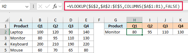
The trick is COLUMNS($A$1:B1). It counts two columns (A and B), so it returns 2, which tells VLOOKUP to grab the second column, Q1.
The start of the range is locked with $A$1, but the end (B1) is not.
So when you copy the formula one cell to the right, it becomes COLUMNS($A$1:C1), which returns 3 and pulls Q2. Copy it again and you get Q3, then Q4.
This saves you from typing 2, 3, 4, 5 by hand into each VLOOKUP.
Pro Tip: If you’re on Excel 365 or 2021, XLOOKUP is cleaner here because it returns the matching value directly without a column index. Use the COLUMNS trick when you’re stuck with VLOOKUP in an older version.
Example 3: Number Columns Sequentially Across a Row
Now let’s look at something handy for headers.
Below is a row of month headers running across columns B to G. I want a running number, 1, 2, 3, and so on, sitting under each month.

I want the first cell to show 1 and each cell to its right to count up by one automatically.
Here is the formula:
=COLUMNS($B$1:B1)

In the first cell, COLUMNS($B$1:B1) counts a single column and returns 1.
Because the start $B$1 is locked and the end grows as you copy right, the next cell reads COLUMNS($B$1:C1) and returns 2, then 3, and so on. You get a clean sequence without typing a single number.
Example 4: Count Columns in a Dynamic Array Spill Range
This next one shows how COLUMNS works with modern spilled results.
Below is an orders table. In a separate area, I’ve used a FILTER formula to pull the orders for one region, and its result spills across several columns starting in cell F2.
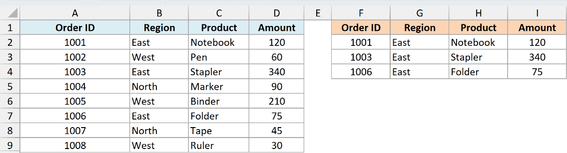
I want to know how many columns the spilled result is, and I want that count to stay correct even if the FILTER output changes.
Here is the formula:
=COLUMNS(F2#)
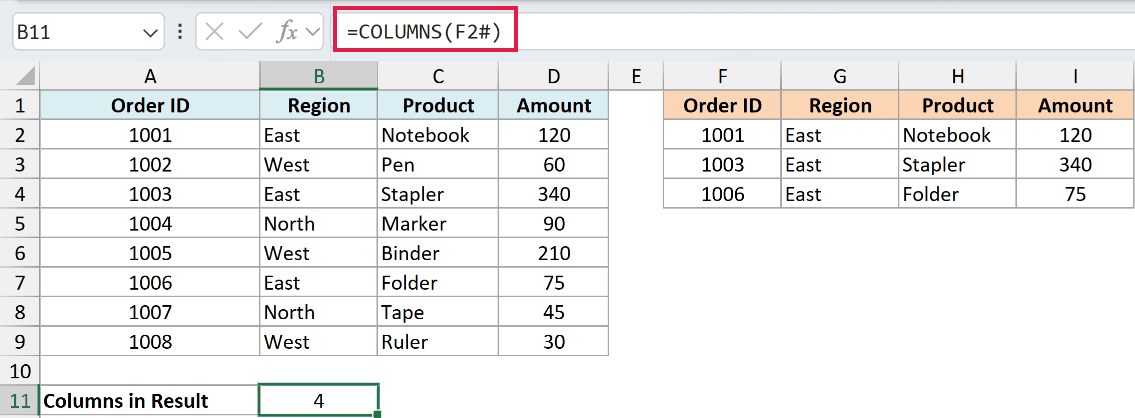
The F2# part is the spill reference. The # tells Excel to use the whole spilled range that starts in F2, however wide it happens to be.
Since the FILTER result has four columns here, COLUMNS returns 4. If you later change FILTER to return more or fewer columns, this count updates on its own.
The spill reference and FILTER are available in Excel 365 and Excel 2021. In older versions you’d point COLUMNS at a fixed range instead.
Example 5: Count the Total Number of Cells in a Range
Let’s finish with a quick calculation you can build using COLUMNS.
Below is a block of data sitting in the range A2:E11. I want the total number of cells it contains.
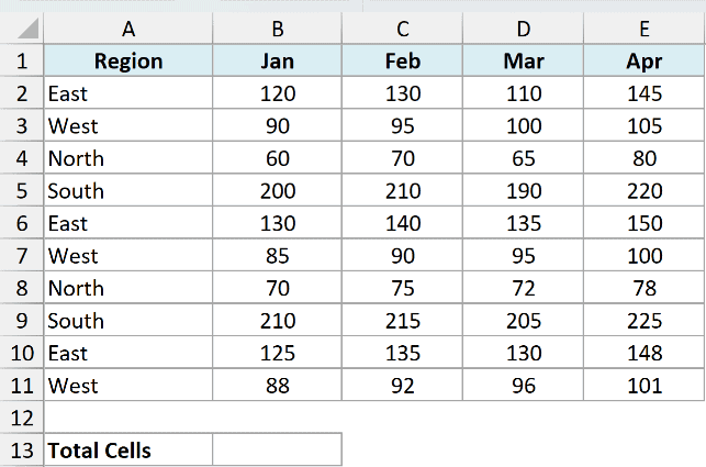
I want to multiply the number of rows by the number of columns to get the total cell count in one formula.
Here is the formula:
=ROWS(A2:E11)*COLUMNS(A2:E11)
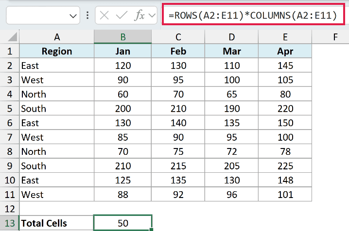
Here, the ROWS function returns 10 (the range is 10 rows tall) and COLUMNS returns 5 (it’s 5 columns wide). Multiplying them gives 50, the total number of cells in the range.
This counts every cell in the range, including blanks. The status bar’s Count can exclude blank cells, so it may show a smaller number.
Tips & Common Mistakes
- COLUMNS is not COLUMN. COLUMNS counts how many columns are in a range. COLUMN returns the column number of a reference. If your result looks off by a lot, check which one you typed.
- Rows don’t matter. COLUMNS only measures width.
COLUMNS(A1:C1)andCOLUMNS(A1:C500)both return 3, so don’t expect it to reflect how tall your data is. - You must give it a valid reference or array. Passing a single cell like
=COLUMNS(A1)returns 1, which is correct but rarely useful. Point it at the actual range you want to measure. - Anchor the reference for a running count. The copy-across tricks in Examples 2 and 3 only work if the start of the range is locked with dollar signs (
$A$1) and the end is left relative. Forget the anchor and the count won’t increment properly.
COLUMNS is one of those small functions that quietly makes bigger formulas smarter. On its own it just counts columns, but paired with VLOOKUP, ROWS, or a spilled array, it saves you from hard-coding numbers that break the moment your data shifts.
Try it the next time you catch yourself counting columns by hand or typing a column index into a lookup.
Other Excel Articles You May Also Like:
