COLUMN Function in Excel

If you want Excel to tell you the column number of a cell or a range, the COLUMN function is the quickest way to get it. Hand it a reference like C2 and it returns 3, because C is the third column.

It looks basic, but COLUMN quietly powers a lot of useful formulas, from building dynamic lookup indexes to converting column letters to numbers.

In Excel 365, you can also feed COLUMN a range and it spills the column numbers into a horizontal array across the cells to the right.

In this article, I’ll show you how to use the COLUMN function in Excel with a handful of practical examples.

COLUMN Function Syntax

Here is the syntax of the COLUMN function:

=COLUMN([reference])

• reference (optional) – the cell or range of cells you want the column number for. Leave it out and COLUMN returns the column number of the cell that holds the formula.

The COLUMN function works in every version of Excel, including Microsoft 365, Excel 2024, 2021, 2019, 2016, older versions, and Excel on the web.

When to Use the COLUMN Function

Use the COLUMN function when you need to:

• Find the numeric position of a column, so you can feed it into another formula
• Build an incrementing column index for VLOOKUP that you drag across
• Create a quick 1-to-N sequence across a row from one formula
• Apply logic to every Nth column with MOD, like totaling quarter-end months or shading alternate columns
• Convert a column letter like AW to its column number, and turn column numbers back into letters

Let me show you a few practical examples of how this works.

Example 1: Get the Column Number of a Cell Reference

Let’s start with the simplest case.

Below is a small product table, with the product name in column A, the category in column B, the price in column C, and the stock count in column D.

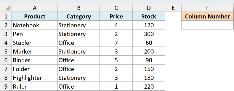
I want to confirm which column number the Price column (column C) sits in.

Here is the formula:

=COLUMN(C2)

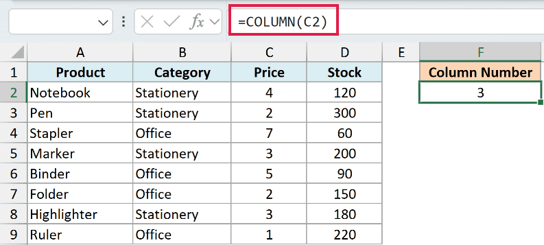
Since column C is the third column in the worksheet, COLUMN returns 3.

Notice that COLUMN only cares about the column, not the row. So =COLUMN(C2) and =COLUMN(C100) both return 3.

Example 2: Return the Column Number of the Current Cell

Here’s a handy variation.

If you leave the reference out entirely, COLUMN returns the column number of the cell the formula is sitting in. There’s no dataset needed here, so I’ll type the formula on a blank sheet.

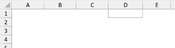
I want to know the column number of the cell where I’m typing, which in this case is cell D1.

Here is the formula:

=COLUMN()

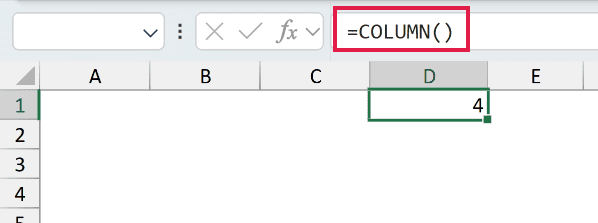
Because the formula is in column D, COLUMN returns 4.

This empty form is the building block for the alternate-column shading trick in Example 6. If you copy the formula to another column, the result updates to match its new position.

Example 3: Spill Column Numbers Across a Range

Now let’s use the modern dynamic array behavior.

When you give COLUMN a range in Excel 365, it spills the column number of every cell in that range into a horizontal array. Again, no dataset is needed, so I’ll do this on a blank sheet.

I want a quick horizontal sequence from 1 to 8 in a single formula.

Here is the formula:

=COLUMN(A1:H1)

Because the range starts at column A (1) and runs through column H (8), the formula spills the numbers 1 through 8 across A1:H1, including the formula cell.

This is a fast way to generate a 1-to-N sequence you can drop inside a bigger formula. It always starts at 1 as long as the range begins in column A.

Pro Tip: In Excel 2019 and earlier, select A1:H1 first, type =COLUMN(A1:H1), then press Ctrl+Shift+Enter. Otherwise, the formula returns only 1. The automatic spill works in Excel 365, 2024, 2021, and Excel for the web.

Example 4: Use COLUMN for a Dynamic VLOOKUP Column Index

This is where COLUMN really earns its keep.

Below is a table of quarterly sales, with the employee name in column A and the four quarters in columns B to E. In cell G2, under an Employee header, I’ve typed the name I want to look up.

I want to pull all four quarters for that employee across a row, using one formula I can drag to the right.

Here is the formula:

=VLOOKUP($G$2,$A$2:$E$7,COLUMN(B1),FALSE)

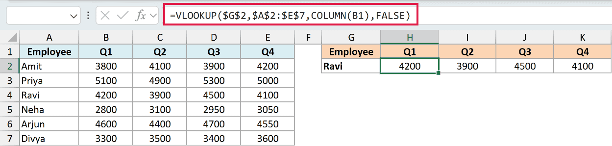
How this formula works:

• VLOOKUP needs a column index number to know which column of the table to return.
• Instead of hard-coding 2, then 3, then 4, then 5, I use COLUMN(B1), which returns 2.
• As you drag the formula to the right, COLUMN(B1) becomes COLUMN(C1), COLUMN(D1), and so on, so the index climbs to 3, 4, and 5 on its own.
• That means one formula copies across and pulls Q1, Q2, Q3, and Q4 without you touching the index.

You can build the same self-adjusting index a couple of other ways. The MATCH function can find a column’s position straight from its header text. And INDEX can return an entire row in one formula, which pairs nicely with MATCH.

Pro Tip: In Excel 365, 2024, 2021, and Excel for the web, you can skip the index counting altogether. The XLOOKUP function returns multiple columns at once, so =XLOOKUP($G$2,$A$2:$A$7,$B$2:$E$7) spills all four quarters in a single formula. Use the COLUMN approach when you’re on an older version that only has VLOOKUP.

Example 5: Sum Every Nth Column with COLUMN and MOD

Let’s step it up with a more advanced use case.

Below I have one product’s monthly sales laid out across a single row, with January in column B through December in column M.

I want the total of only the quarter-end months (March, June, September, and December) without selecting them by hand.

Here is the formula:

=SUMPRODUCT((MOD(COLUMN(B2:M2)-COLUMN(B2),3)=2)*B2:M2)

How this formula works:

• COLUMN(B2:M2) returns the column numbers 2 through 13, one for each month.
• Subtracting COLUMN(B2) rebases those to 0 through 11, so each month gets a position number.
• MOD(...,3)=2 is TRUE only at positions 2, 5, 8, and 11, which are March, June, September, and December.
• SUMPRODUCT multiplies those TRUE/FALSE flags by the sales figures and adds up the survivors, giving 610.

To total a different set, change the step (the 3) and the offset (the 2) to match the pattern you want.

Example 6: Shade Alternate Columns Using COLUMN

Here’s a formatting trick that uses COLUMN inside a conditional formatting rule.

Below is a wide table where reading across the rows gets a little hard on the eyes.

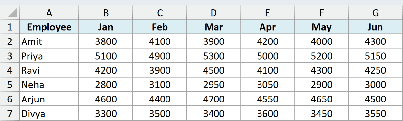
I want to shade every other column so the table is easier to scan.

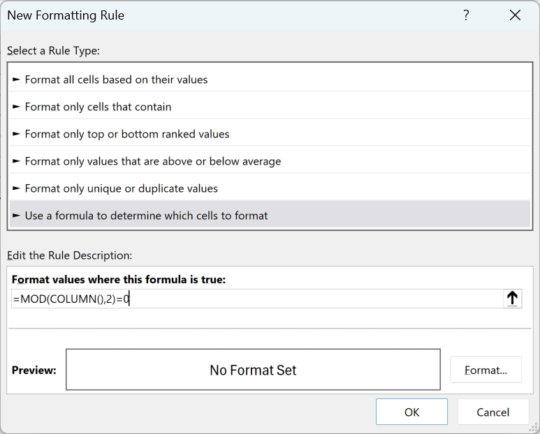
1. Select the data range A2:G7, go to the Home tab, click Conditional Formatting, then New Rule. In the dialog, choose “Use a formula to determine which cells to format.”

2. Enter the formula below in the “Format values where this formula is true” field.

=MOD(COLUMN(),2)=0

3. Click the Format button, go to the Fill tab, pick the color you want (light green here), and click OK.

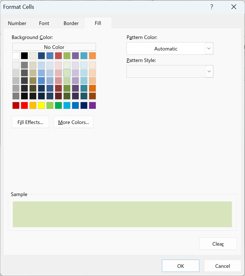
4. Click OK to apply the rule. Every other column gets the fill.

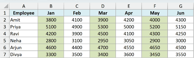
As the rule checks each cell, COLUMN() returns that cell’s column number. MOD(...,2)=0 is TRUE for even columns, so columns B, D, and F get the fill and the others stay clear.

Swap the formula to =MOD(COLUMN(),2)=1 if you’d rather shade the odd columns instead.

Example 7: Convert Column Letters to Numbers and Numbers to Letters

COLUMN can turn AW into 49, and ADDRESS with SUBSTITUTE can turn 49 back into AW.

Below I have column letters in A2:A9 and their matching numbers in D2:D9, with an empty spacer column between the two tables.

Column B has a Column Number header, and column E has a Column Letter header. The results will go below these headers.

I want to convert the letters in A2:A9 to column numbers in one formula, with the results starting in B2.

Here is the formula:

=COLUMN(INDIRECT(A2:A9&"1"))

The formula spills the column numbers into B2:B9. AW becomes 49, and Excel’s last column, XFD, becomes 16,384.

How this formula works:

• A2:A9&"1" adds a row number to each letter, building text such as “AW1”.
• The INDIRECT function turns that text into a real cell reference.
• COLUMN returns the column number of each reference, so AW1 gives us 49.

For a single column like AW, you can use a direct reference:

=COLUMN(AW1)

This returns 49 without needing INDIRECT.

Now let’s go the other way. The column numbers are in D2:D9, and column E is ready for the letters.

I want to turn those numbers back into column letters, with the results starting in E2.

Here is the formula:

=SUBSTITUTE(ADDRESS(1,D2:D9,4),"1","")

The formula spills the letters into E2:E9, so 49 becomes AW.

How this formula works:

• ADDRESS(1,D2:D9,4) builds a cell address for each number, using row 1.
• The 4 gives a relative reference without $ signs, so column 49 becomes “AW1”.
• SUBSTITUTE removes the “1”, leaving “AW”. Since the row is always 1 and column letters contain no digits, only the row number is removed.

The two range formulas above spill in Excel 365, 2024, 2021, and Excel for the web.

Pro Tip: In Excel 2019 and earlier, use the single-cell versions below and copy each formula down to row 9.

In B2, use:

=COLUMN(INDIRECT(A2&"1"))

In E2, use:

=SUBSTITUTE(ADDRESS(1,D2,4),"1","")

To get the letter of a cell’s own column, use COLUMN inside ADDRESS:

=SUBSTITUTE(ADDRESS(1,COLUMN(D2),4),"1","")

This returns “D”, because COLUMN(D2) gives us 4 and ADDRESS uses that number to build “D1”.

COLUMN vs COLUMNS in Excel

These two get mixed up constantly because the names look almost identical, but they answer different questions.

COLUMN returns the column number (or numbers) of a reference. So =COLUMN(B1) returns 2.

COLUMNS counts how many columns are in a range. So =COLUMNS(B1:E1) returns 4, because that range is four columns wide.

A simple way to remember it: COLUMN tells you which column, COLUMNS tells you how many columns. You can read more in my guide to the COLUMNS function.

Tips & Common Mistakes

• COLUMN returns a number, not a letter. =COLUMN(D2) gives you 4, not “D”. To get the column letter, you can combine it with the ADDRESS and SUBSTITUTE functions, as shown in Example 7.
• Don’t confuse it with COLUMNS. COLUMN returns the position, COLUMNS returns the count. Reach for the wrong one and your formula quietly returns the wrong number.
• The empty form follows the formula. =COLUMN() returns the column of whatever cell it lives in, so it changes if you move or copy the formula somewhere else.
• Older versions don’t spill. In Excel 2019 and earlier, select the output cells, type the formula, then press Ctrl+Shift+Enter. Otherwise, it returns only the leftmost column number. In Excel 365, 2024, 2021, and Excel for the web it spills on its own.
• No multi-area references. COLUMN can’t handle a reference that spans separate areas, like =COLUMN((A1,C1)), so keep it to a single continuous range.

The COLUMN function looks basic on its own, but it does a lot of quiet work inside bigger formulas, from dynamic lookups to totaling every Nth column.

Once you know it returns a column’s numeric position, you’ll spot plenty of places to use it.

Give these examples a try in your own workbook. Next time you’re about to hard-code a column number, see if a COLUMN formula fits instead.

List of All Excel Functions

Other Excel Articles You May Also Like:

• Excel ROW Function | Formula Examples + FREE Video
• 10 VLOOKUP Examples For Beginner & Advanced Users
• ROWS Function in Excel (6 Examples)
• OFFSET Function in Excel (7 Examples)
• 20 Advanced Excel Functions and Formulas (for Excel Pros)
• How to Return Cell Address Instead of Value in Excel (Easy Formula)
• INDEX & MATCH Functions Combo in Excel (10 Easy Examples)
• VLOOKUP Not Working? (10 Common Fixes)