
When using lookup formulas in Excel (such as VLOOKUP, XLOOKUP, or INDEX/MATCH), the intent is to find the matching value and get that value (or a corresponding value in the same row/column) as the result.
But in some cases, instead of getting the value, you may want the formula to return the cell address of the value. A cell address is the column letter and row number of a cell, such as C6.
This could be especially useful if you have a large data set and you want to find out the exact position of the lookup formula result.
There are some functions in Excel that are designed to do exactly this.
In this tutorial, I will show you how you can find and return the cell address instead of the value in Excel using simple formulas.
I’ll also show you how to get the address of every matching cell when the value shows up more than once.
Follow along with the example file
Return Cell Address Instead of Value Excel.xlsx
Lookup and Return Cell Address Using CELL and XLOOKUP
Let’s start with the shortest formula, which works in Excel 365, 2024, and 2021.
The ADDRESS function was made specifically to give you a cell address (I cover it in the next section), but there is another function that also does this.
It’s called the CELL function (and it can give you a lot more information about the cell than the ADDRESS function).
Below is the syntax of the CELL function:
=CELL(info_type, [reference])
where:
- info_type: the information about the cell you want. This could be the address, the column number, the file name, etc.
- [reference]: Optional argument where you can specify the cell reference for which you need the cell information.
Now, let’s see an example where you can use this function to look up and get the cell reference.
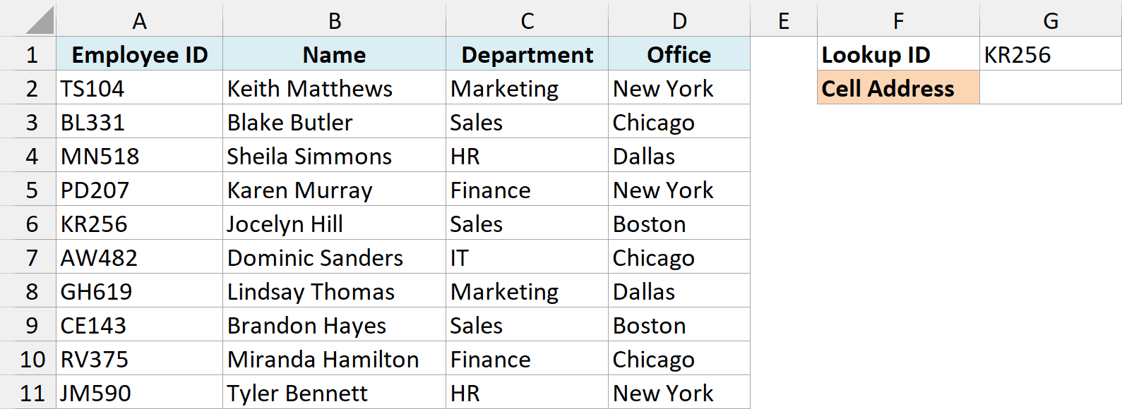
Below is a list of employees with their ID, name, department, and office, and I want the address of the cell that holds the department for the employee ID in cell G1 (KR256) in cell G2.
Below is the formula that will do this:
=CELL("address",XLOOKUP(G1,A2:A11,C2:C11))
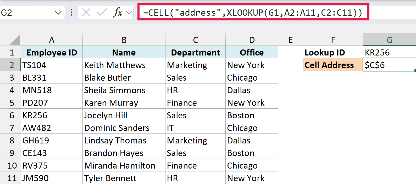
The above formula is quite straightforward.
How this formula works:
- XLOOKUP(G1,A2:A11,C2:C11) – This looks for KR256 in A2:A11 and returns the matching cell from the Department column, which is C6 (it holds “Sales”).
- CELL(“address”, …) – This gives you the address of that cell as text, which is $C$6.
Now here is the secret to why it works.
The XLOOKUP formula returns the lookup value when you give it all the necessary arguments. But at the same time, it would also return the cell reference of that resulting cell.
In our example, the XLOOKUP formula returns “Sales” as the resulting value, but at the same time, you can also use it to give you the cell reference of that value instead of the value itself.
Normally, when you enter the XLOOKUP formula in a cell, it returns the value because that is what it’s expected to do. But in scenarios where a cell reference is required, the XLOOKUP formula will give you the cell reference.
In this example, that’s exactly what it does. The second argument of CELL needs a cell reference, so XLOOKUP hands it the cell C6 instead of the value “Sales”.
This is also why the trick doesn’t work with VLOOKUP. VLOOKUP can only return a value, so Excel won’t even accept a formula like =CELL(“address”,VLOOKUP(…)).
And the best part about using this formula is that it is not tied to the first cell in the worksheet.
This means that you can select any data set (which could be anywhere in the worksheet), use XLOOKUP to do a regular lookup, and it would still give you the correct address.
And if you insert an additional row or column, the formula would adjust accordingly to give you the correct cell address.
That’s not true for every method. The simple ADDRESS formula in the next section counts positions from row 1, so it gives the wrong cell when your data starts lower down or when you insert rows above it.
If your data is on a different sheet, the result also includes the file and sheet name, such as [Book1.xlsx]Data!$C$6.
If you plan to copy this formula down a long list, keep in mind that Microsoft lists CELL among the functions that can recalculate every time anything in the workbook changes.
With a few lookups, you won’t notice it. But with thousands of these formulas, every edit makes Excel recalculate all of them, which can slow the workbook down, so use the ADDRESS method in the next section instead.
If you are using Excel 2019 or earlier, use the below formula instead (it’s in cell G3 of the example file):
=CELL("address",INDEX(C2:C11,MATCH(G1,A2:A11,0)))
Here, the MATCH function finds the position of KR256 in A2:A11, and I have used the INDEX formula to get the department for the employee ID KR256.
And then simply wrapped it within the CELL function and asked it to return the cell address of this value that I get from the INDEX formula. INDEX returns a cell reference just like XLOOKUP does, so you get the same $C$6.
Sometimes you don’t need the full address, just the row number where the match is. In that case, wrap the same XLOOKUP in the ROW function (this one is in cell G4 of the example file):
=ROW(XLOOKUP(G1,A2:A11,C2:C11))
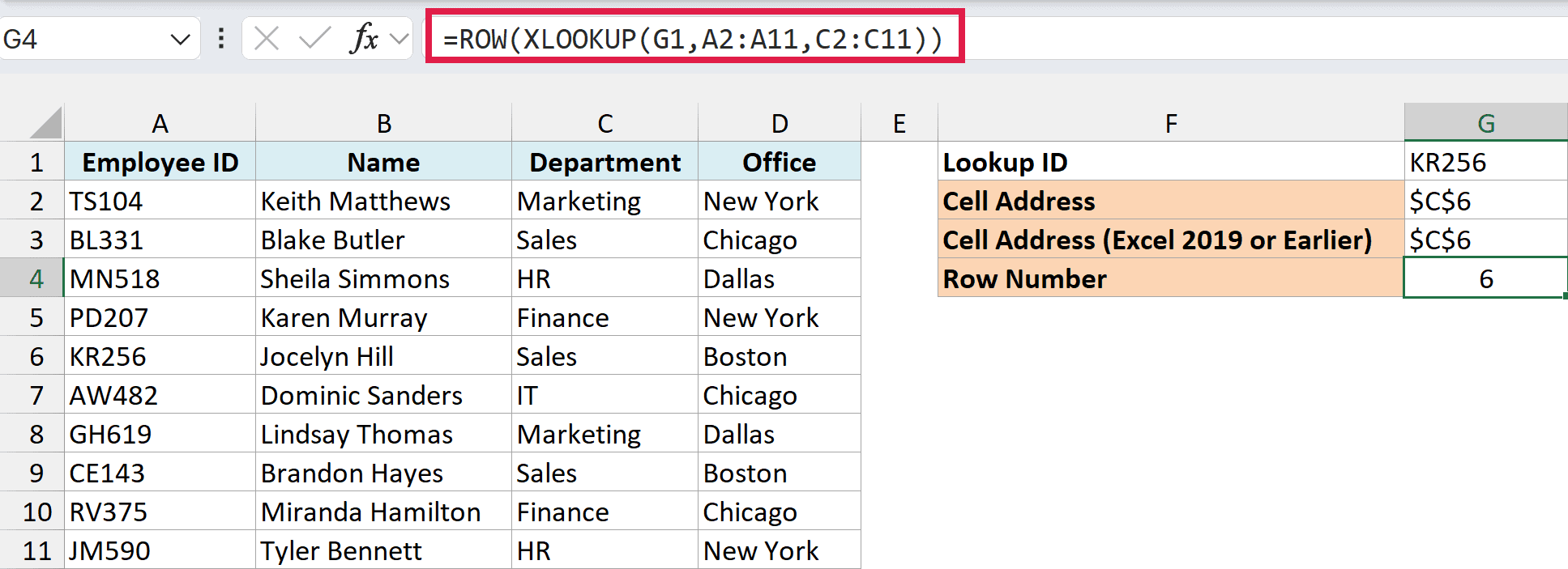
This returns 6, which is the row of the worksheet where KR256 sits. Since XLOOKUP hands ROW the actual cell, you get the real row number even if your data doesn’t start in row 1.
If you are using Excel 2019 or earlier, enter the below formula in cell G4 instead:
=ROW(INDEX(C2:C11,MATCH(G1,A2:A11,0)))
Lookup and Return Cell Address Using the ADDRESS Function
Now let’s look at the function that was built for this job.
The ADDRESS function in Excel is meant to do exactly this. It takes the row and the column number and gives you the cell address of that specific cell.
Below is the syntax of the ADDRESS function:
=ADDRESS(row_num, column_num, [abs_num], [a1], [sheet_text])
where:
- row_num: Row number of the cell for which you want the cell address
- column_num: Column number of the cell for which you want the address
- [abs_num]: Optional argument where you can specify whether you want the cell reference to be absolute, relative, or mixed.
- [a1]: Optional argument where you can specify whether you want the reference in the R1C1 style or A1 style
- [sheet_text]: Optional argument where you can specify a sheet name that you want to add along with the cell address (for example, Data!$C$6)
Now, let’s take an example and see how this works.
Below is the same list of employees with their ID, name, department, and office, and I want the address of the cell that holds the department for the employee ID in cell G1 (KR256) in cell G2.
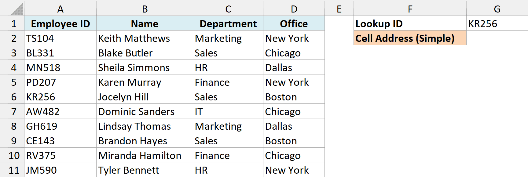
Below is the formula that will do this:
=ADDRESS(MATCH(G1,A1:A11,0),3)
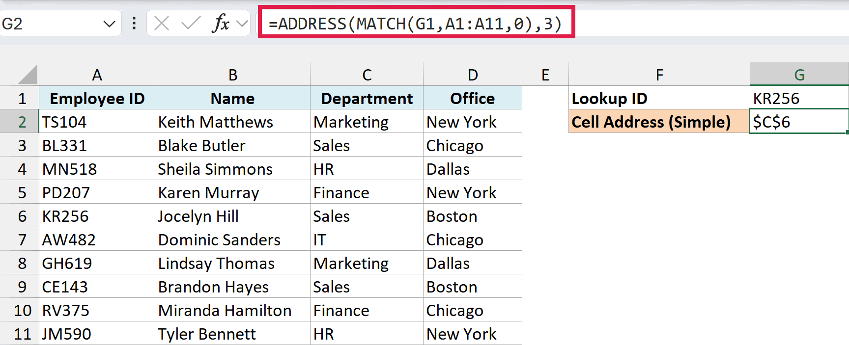
In the above formula, I have used the MATCH function to find out the row number that contains the given employee ID. Since the range A1:A11 starts in row 1, the position MATCH returns (6) is also the row number.
And since the department is in column C, I have used 3 as the second argument.
This formula works great, but it has one drawback: it won’t work if you add a row above the dataset or a column to the left of the dataset. Instead of showing an error, it quietly keeps showing the old address.
This is because when I specify the second argument (the column number) as 3, it’s hard-coded and won’t change.
In case I add any column to the left of the dataset, the formula would count 3 columns from the beginning of the worksheet and not from the beginning of the dataset.
The row has the same problem. MATCH counts from the top of the range A1:A11, so once a row is added above the data, that position is no longer the row number.
You can see this in the example file. Insert a row above the data and the formula still says $C$6, even though the department for KR256 has moved down to C7.
So, if you have a fixed dataset and need a simple formula, this will work fine.
But if you need this to be more fool-proof, use the below formula instead:
=ADDRESS(MATCH(G1,A:A,0),COLUMN(C:C))
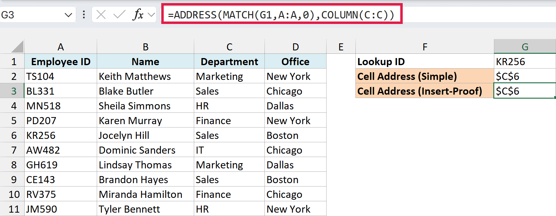
How this formula works:
- MATCH(G1,A:A,0) – This looks for KR256 in the whole of column A. Since a whole column always starts at row 1, the position it returns (6) is always the actual row number, even after you insert rows above the data.
- COLUMN(C:C) – This returns 3, the column number of column C. If you insert a column to the left, the reference moves to D:D and this becomes 4 on its own.
- ADDRESS – This turns row 6 and column 3 into $C$6.
Since this formula searches the whole of column A, make sure the employee ID doesn’t appear anywhere else in that column. If it does, MATCH stops at the first one it finds.
By default, ADDRESS gives you an absolute reference with dollar signs ($C$6). If you want a plain C6, use 4 as the third argument:
=ADDRESS(MATCH(G1,A:A,0),COLUMN(C:C),4)
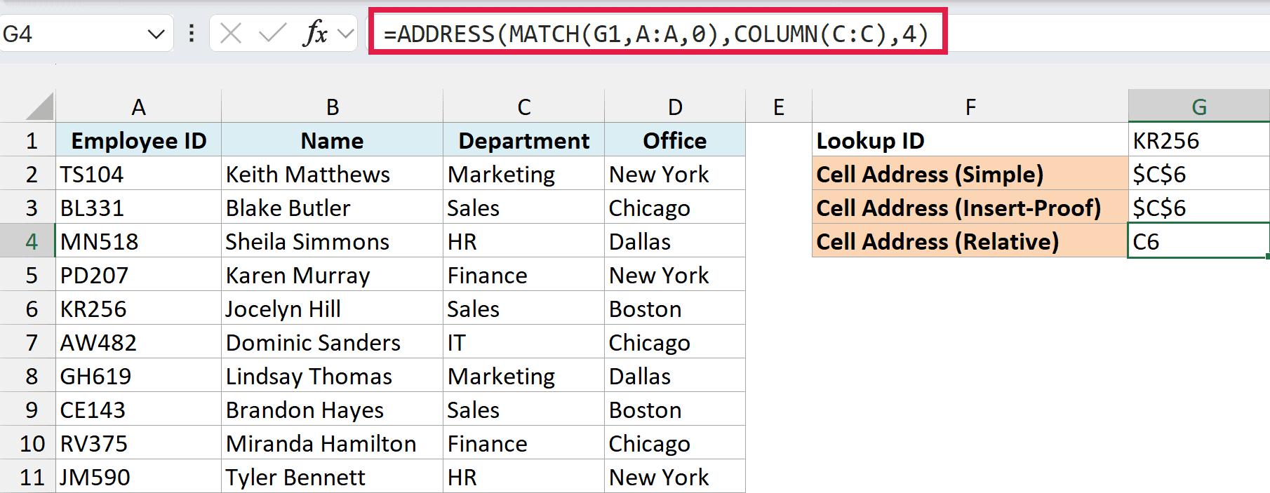
The ADDRESS and MATCH functions work in all Excel versions, so this method is a good pick if your file needs to work in an older version.
Return the Cell Address of Every Match (Not Just the First)
Both the methods above stop at the first match, so if the value you’re looking for shows up more than once, you only get the first address.
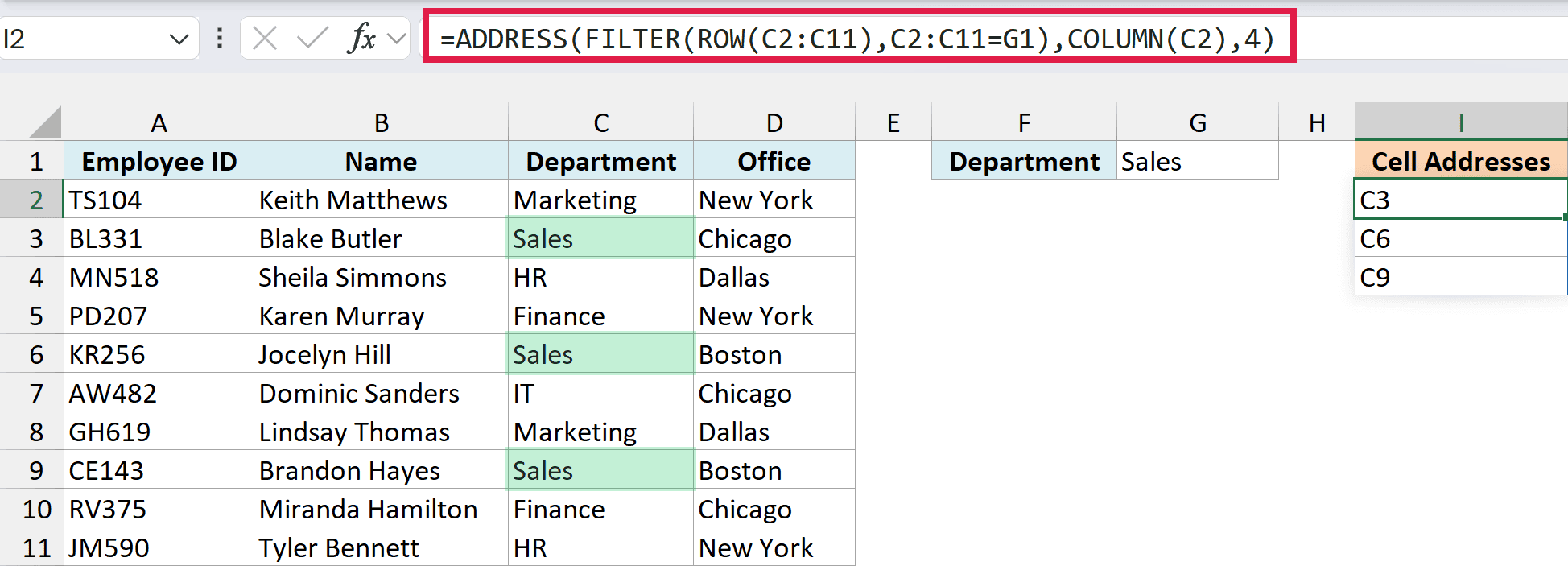
Below is the same list of employees, and I want the addresses of all the cells in the Department column that say Sales (the department is typed in cell G1), listed in column I.
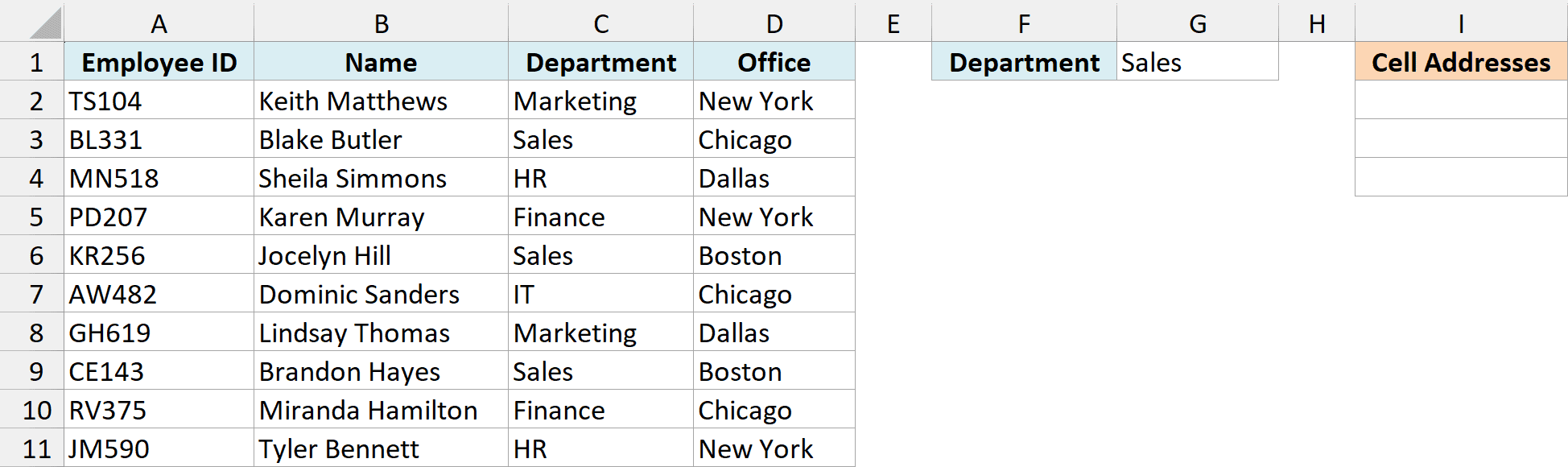
Here is the formula that will do this:
=ADDRESS(FILTER(ROW(C2:C11),C2:C11=G1),COLUMN(C2),4)
How this formula works:
- ROW(C2:C11) – This gives the row numbers of the Department column, 2 to 11.
- FILTER(ROW(C2:C11),C2:C11=G1) – This keeps only the row numbers where the department is Sales, which are 3, 6, and 9.
- COLUMN(C2) – This returns 3, the column number of the Department column.
- ADDRESS(…,4) – This turns each row number and column 3 into an address, and the 4 makes them plain addresses without dollar signs.
The result is C3, C6, and C9, and the formula spills down on its own, so you don’t need to copy it.
If nothing matches (say G1 has a department that isn’t in the list), FILTER returns a #CALC! error. To show a friendlier message instead, wrap the formula in the IFERROR function:
=IFERROR(ADDRESS(FILTER(ROW(C2:C11),C2:C11=G1),COLUMN(C2),4),"Not found")
This formula needs the FILTER function, which is available in Excel 365, 2024, and 2021.
If you are using Excel 2019, enter the below formula in cell I2 instead and confirm it with Ctrl + Shift + Enter. It uses the TEXTJOIN function to list all the addresses in one cell, separated by commas:
=TEXTJOIN(", ",TRUE,IF(C2:C11=G1,ADDRESS(ROW(C2:C11),COLUMN(C2),4),""))
Find the Cell Address of a Value Anywhere in a Table
The formula above searches one column. But sometimes the value you’re looking for could be in any cell of a table, and you want to know every place it shows up.
Below is a weekly shift roster, and I want the addresses of all the shifts that Meredith (the name in cell G1) is working, listed in column I.
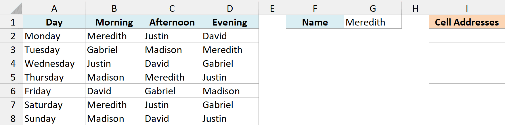
Here is the formula that will do this:
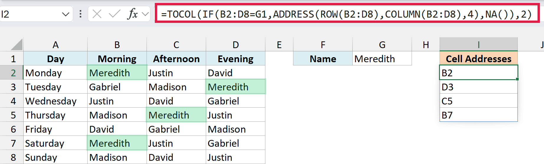
=TOCOL(IF(B2:D8=G1,ADDRESS(ROW(B2:D8),COLUMN(B2:D8),4),NA()),2)
How this formula works:
- ADDRESS(ROW(B2:D8),COLUMN(B2:D8),4) – ROW gives the row numbers 2 to 8 and COLUMN gives the column numbers 2 to 4. ADDRESS pairs every row number with every column number, so you get a grid of addresses (B2, C2, D2, and so on) the same shape as the roster.
- IF(B2:D8=G1,…,NA()) – This keeps the address only where the cell has Meredith, and puts a #N/A error everywhere else.
- TOCOL(…,2) – This turns the grid of results into a single column, and the 2 tells it to skip the errors. So only Meredith’s addresses are left.
The result is B2, D3, C5, and B7, listed row by row. I’ve used the same trick to list every blank cell in a range in my ADDRESS function tutorial.
This formula needs the TOCOL function, which is only available in Excel 365 and Excel 2024.
If nothing matches, it returns a #CALC! error, and you can wrap it in IFERROR just like the previous formula.
If you are using Excel 2021 or 2019, enter the below formula in cell I2 instead (in Excel 2019, confirm it with Ctrl + Shift + Enter). It lists all the addresses in one cell, separated by commas:
=TEXTJOIN(", ",TRUE,IF(B2:D8=G1,ADDRESS(ROW(B2:D8),COLUMN(B2:D8),4),""))
So these are some simple formulas that you can use to look up and find and return the cell address instead of the value in Excel.
If you want to take this further, my CELL function tutorial also shows how to get the address of the highest value and how to build a link that jumps straight to a lookup result.
I hope you found this tutorial useful.
Other Excel tutorials you may also like:
- Lookup and Return Values in an Entire Row/Column in Excel
- Find the Last Occurrence of a Lookup Value a List in Excel
- Lookup the Second, the Third, or the Nth Value in Excel
- How to Reference Another Sheet or Workbook in Excel
- Lookup and Return Multiple Values in One Cell in Excel
- How to Use XLOOKUP with Multiple Criteria in Excel