

If you want to find out which row a cell sits in, or build a list of numbers that keeps itself in order, the ROW function is what you reach for.
It returns the row number of a reference, or of the cell that holds the formula when you leave the reference out.
In Excel 365, you can also feed ROW a whole range and the row numbers spill into the cells below.
In this article, I’ll show you how to use ROW in Excel, from a plain row-number lookup to serial numbers, alternate-row logic, and summing every nth row.
Follow along with the example file
ROW Function Examples.xlsx
ROW Function Syntax
Here is what the ROW function looks like:
=ROW([reference])
Here is what the one argument means:
- [reference] is optional. It’s the cell or range whose row number you want. Leave it out and ROW returns the row number of the cell the formula sits in.
ROW works in Excel for Microsoft 365, Excel 2024, 2021, 2019, 2016, and older versions, plus Excel on the web. The spilling behavior in Example 2 needs Excel 365 or 2021.
When to Use the ROW Function
Use the ROW function when you need to:
- Get the worksheet row number of a specific cell.
- Build serial numbers that renumber themselves when you delete rows (or add rows and copy the formula down).
- Drive alternate-row shading and banding logic with MOD.
- Sum or pull out values from every nth row.
- Feed a growing counter into INDEX and other array formulas.
Let me show you a few practical examples of how this works.
Example 1: Get the Row Number of a Cell
Let’s start with the simplest thing ROW does.
Below is a short list of product codes in column A, starting in cell A2.
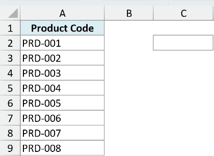
I want to know the worksheet row number of the code sitting in cell A5.
Here is the formula:
=ROW(A5)
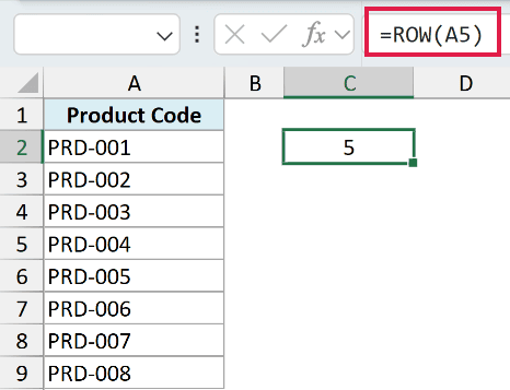
Here, ROW looks at the reference A5 and hands back the number 5, because A5 is on the fifth row of the worksheet. Point it at any cell and you get that cell’s row number.
You can also skip the reference entirely and let ROW report its own location.
=ROW()
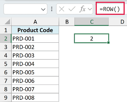
With no reference, ROW returns the row number of the cell holding the formula. Typed into cell C2, it returns 2. This “own row” trick is what powers the serial-number formula in Example 3.
Example 2: Spill a Column of Row Numbers
Here’s where Excel 365 makes ROW more useful.
Below I have ten podcast episode titles in the range A2:A11.
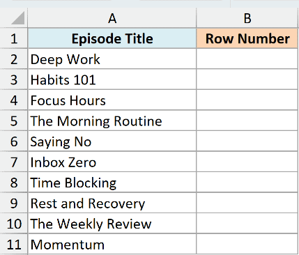
I want the worksheet row number of every one of those cells, all from a single formula.
Here is the formula:
=ROW(A2:A11)
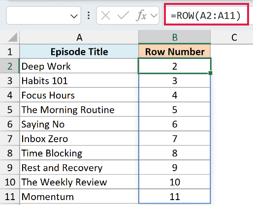
Fed a range, ROW returns an array of every row number in it. In Excel 365 that array spills down the column, so one formula in B2 fills B2:B11 with 2, 3, 4, all the way to 11.
Pro Tip: The numbers above match the sheet rows (2 to 11), not a clean 1 to 10. For a list that starts at 1, use =ROW(1:10) or the newer =SEQUENCE(10) instead.
In Excel 2019 and earlier, this same formula returns only the first row number (2), since those versions don’t spill. You can also force a single value in 365 with =@ROW(A2:A11), which returns 2.
Example 3: Build Serial Numbers With the ROW Function
This is one of the most common reasons people reach for ROW.
Below is a table of support tickets, with the ticket ID in column B and its priority in column C. Column A is an empty serial-number column.
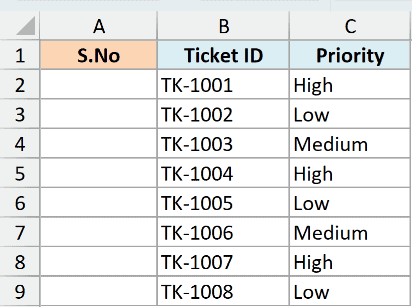
I want a serial number in column A that always starts at 1 and re-numbers itself if I delete a ticket.
Here is the formula I put in cell A2 and fill down:
=ROW()-1
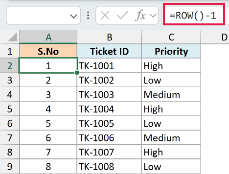
ROW() returns the sheet row number, and subtracting 1 accounts for the header in row 1. So A2 shows 1, A3 shows 2, and so on. Delete a ticket and the formulas below recalculate, so the numbering stays 1, 2, 3 with no gaps.
We keep this one per-row (filled down) rather than spilling it, because each serial number needs to sit next to its own ticket. If you want the full rundown of ways to do this, see how to number rows in Excel.
Pro Tip: The -1 offset assumes your data starts in row 2. If your table starts lower, change the number so the first serial comes out as 1 (for a header in row 3, use =ROW()-3).
Example 4: Flag Every Other Row Using ROW and MOD
The ROW function is what makes alternate-row formatting possible.
Below is a table of daily temperature readings, with the date in column A and the reading in column B.
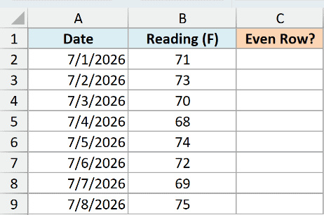
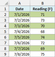
I want a TRUE/FALSE flag that turns on for every even row, so I can shade alternate rows.
Here is the formula:
=MOD(ROW(),2)=0
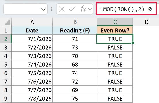
MOD(ROW(),2) divides the current row number by 2 and returns the remainder, which is 0 on even rows and 1 on odd rows. Testing it against 0 gives TRUE on every even row and FALSE on the rest.
Drop this exact test into a conditional formatting formula rule instead of a helper column and Excel shades every other row for you. It leans on the same idea as the MOD function.
Example 5: Sum Every Nth Row With ROW and SUMPRODUCT
Let’s step it up with a more advanced use.
Below I have twelve rainfall readings, with the day in column A and the reading in B2:B13.
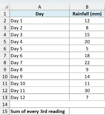
I want to add up only every 3rd reading, which lands on rows 2, 5, 8, and 11.
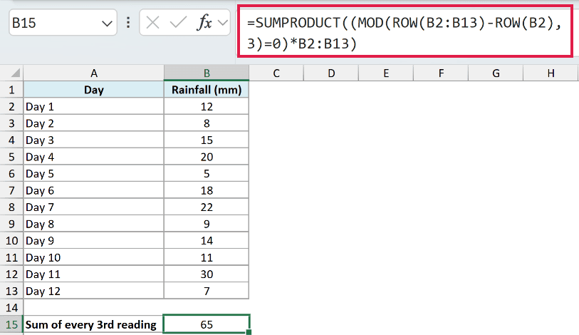
Here is the formula:
=SUMPRODUCT((MOD(ROW(B2:B13)-ROW(B2),3)=0)*B2:B13)
How this formula works:
- ROW(B2:B13) builds the array {2;3;4;…;13}, one row number per cell.
- Subtracting ROW(B2) shifts that to {0;1;2;…}, so the count starts at 0 no matter where the data sits.
- MOD(…,3)=0 is TRUE at every 3rd position (0, 3, 6, 9) and FALSE everywhere else.
- Multiplying by B2:B13 keeps only the matching values, and SUMPRODUCT adds them up.
With readings of 12, 20, 22, and 11 on those rows, the formula returns 65.
Example 6: Pull Every Nth Item Using ROW and INDEX
Here’s a handy one when you want to sample a long list.
Below is a list of 18 survey respondent IDs in the range A2:A19.
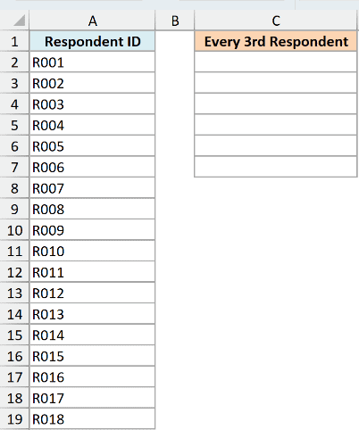
I want to pull every 3rd respondent into a new column, starting from the first one.
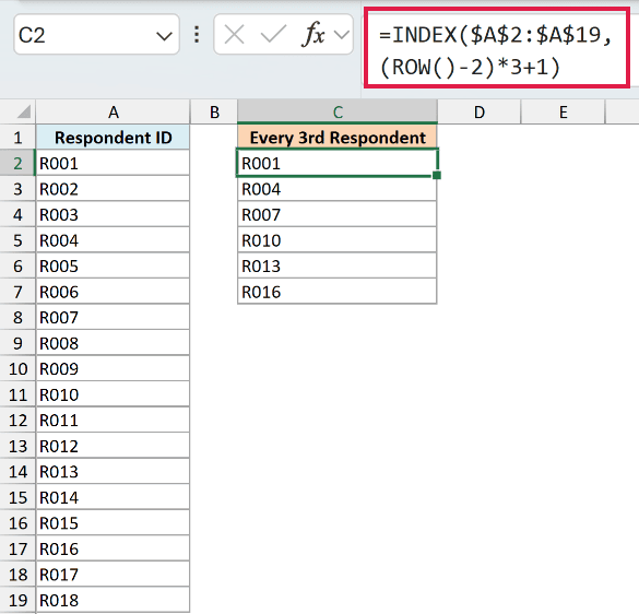
Here is the formula I put in cell C2 and fill down:
=INDEX($A$2:$A$19,(ROW()-2)*3+1)
How this formula works:
- (ROW()-2) turns the formula’s own row into a counter that reads 0, 1, 2, and so on as you fill down.
- Multiplying by 3 and adding 1 turns that counter into the positions 1, 4, 7, 10, and so on.
- INDEX pulls the item at that position out of the list.
Fill it down and you get the 1st, 4th, 7th, 10th, 13th, and 16th IDs. Once the positions run past the list, INDEX returns a #REF! error, so fill only as far as you need.
Pro Tip: Change the 3 to sample a different interval (5 for every 5th item), and change the -2 to match the row where your first formula sits.
Tips & Common Mistakes
- Don’t confuse ROW with ROWS. ROW returns a row number, while ROWS counts how many rows are in a range. =ROW(A2:A11) gives 2 (or spills 2 to 11 in 365), but =ROWS(A2:A11) gives 10.
- Leaving out the reference returns the formula cell’s own row, not row 1. That’s the point, but remember the result changes if you move the formula to a different row.
- Spilling needs a modern version. In Excel 365 and 2021, =ROW(A2:A11) spills the full array. In Excel 2019 and earlier it returns only the first row number, and you’d need Ctrl+Shift+Enter for the array behavior.
- Serial numbers made with ROW re-sequence on their own, which beats typing numbers by hand after every insert or delete (after inserting a row, copy the formula into the new cell, or use an Excel Table so it fills in automatically). Just know they also shift if you sort the data, so paste them as values first if you need the numbers frozen.
The ROW function looks tiny, but it does a lot of quiet work. On its own it just reports a row number, yet paired with MOD, SUMPRODUCT, and INDEX it drives serial numbers, alternate-row shading, and every-nth-row math.
Keep it in mind whenever a formula needs to know where it is on the sheet. I hope you found this tutorial helpful.
Other Excel Articles You May Also Like:
