

If you want the remainder left over after you divide one number by another, the MOD function in Excel is what you’re looking for. It takes a number and a divisor and hands you back whatever is left.
In Excel 365, you can also feed MOD a whole range and the results spill into the cells below.
In this article, I’ll show you how to use MOD with practical examples, from simple remainders to repeating sequences and splitting time.
Follow along with the example file
MOD Function Examples.xlsx
MOD Function Syntax
Here is the syntax of the MOD function:
=MOD(number, divisor)
- number – The number you want to divide.
- divisor – The number you want to divide by. The result comes back with the same sign as this divisor.
When to Use the MOD Function in Excel
Use this function when you need to:
- Get the remainder or leftover after dividing two numbers
- Test whether a number is even or odd
- Add up only the odd or only the even values in a list
- Flag or highlight every Nth row in a table
- Highlight the decimals or the whole numbers in a range
- Build a repeating sequence or rotate items in a cycle
- Pull the seconds out of a time value
Let me show you a few practical examples of how to use MOD in real situations.
Example 1: Get the Remainder After Dividing
Let’s start with a simple example.
Below is a dataset with office supplies in column A and the number of units ordered in column B. These items ship in full boxes of 12.
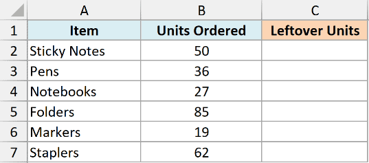
I want to know how many loose units are left over for each product after packing as many full boxes of 12 as possible.
Here is the formula:
=MOD(B2:B7,12)
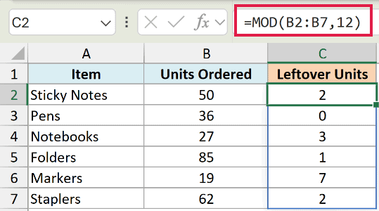
Here, MOD divides each quantity by 12 and returns only the remainder. For 50 units, that’s 2 left over (12 goes in 4 times, leaving 2).
Since this is Excel 365, one formula fed the whole B2:B7 range and the leftovers spilled down the column automatically. No dragging needed.
Pro Tip: MOD gives you the leftover. If you want the number of full boxes instead, use QUOTIENT, like =QUOTIENT(B2,12), which returns the whole-number part of the division.
Example 2: Check if a Number Is Even or Odd
Here’s another practical scenario.
Below is a dataset with attendee names in column A and their assigned seat numbers in column B. Even seats are on one side of the aisle, odd seats on the other.
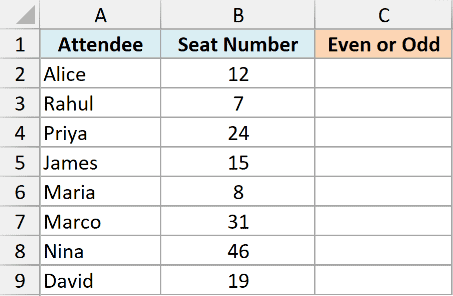
I want to label each seat as Even or Odd so people know which side to walk to.
Here is the formula:
=IF(MOD(B2:B9,2)=0,"Even","Odd")
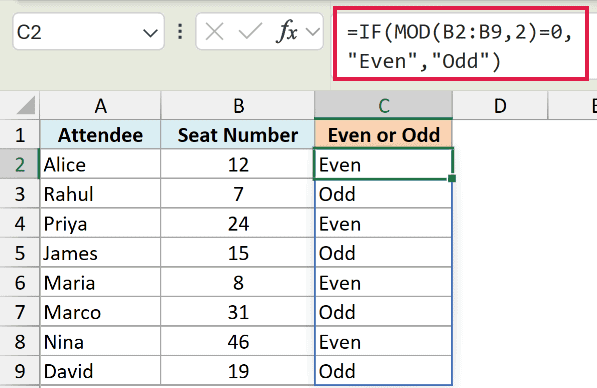
The trick here is dividing by 2. Any even number divides by 2 with no remainder, so MOD returns 0. Any odd number leaves a remainder of 1.
The IF then reads that result and prints “Even” when the remainder is 0 and “Odd” otherwise.
Pro Tip: Excel also has dedicated ISEVEN and ISODD functions that do the even/odd check for you, so =ISEVEN(B2) returns TRUE or FALSE without the MOD.
Example 3: Sum Only the Odd or the Even Numbers
Here’s a handy one for splitting a list by whether the values are odd or even.
Below is a dataset with 10 boxes in column A and the number of items each box holds in column B.
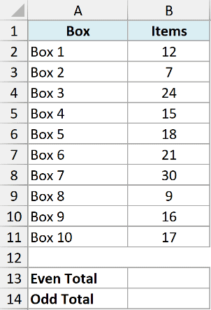
I want to total the boxes that hold an even count separately from the boxes that hold an odd count.
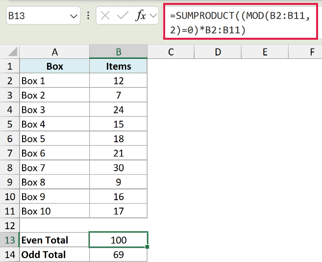
Here is the formula for the even total:
=SUMPRODUCT((MOD(B2:B11,2)=0)*B2:B11)
And here is the formula for the odd total:
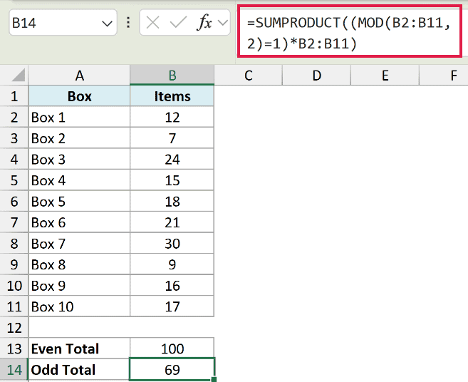
=SUMPRODUCT((MOD(B2:B11,2)=1)*B2:B11)
How this formula works:
MOD(B2:B11,2)returns the remainder for each count, 0 for even and 1 for odd.- The comparison (
=0or=1) turns that into an array of TRUE and FALSE values. - SUMPRODUCT multiplies those flags by the item counts and adds only the matches, so the even total comes to 100 and the odd total to 69.
Pro Tip: In Excel 365 you can get the same split with SUM and a filter, like =SUM(FILTER(B2:B11,MOD(B2:B11,2)=0,0)), which reads a little more plainly. The final 0 returns 0 when no even numbers match.
Example 4: Highlight Every Other Row with MOD
Now let’s use MOD to shade alternating rows so a plain table is easier to read.
Below is a dataset with product names in column A and their prices in column B. I want to shade every other row a light color, without turning the range into an Excel Table.
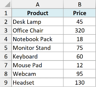
To do this, select the data, go to Home, then Conditional Formatting, then New Rule, and choose the option to use a formula. Enter the formula below.
=MOD(ROW(),2)=0
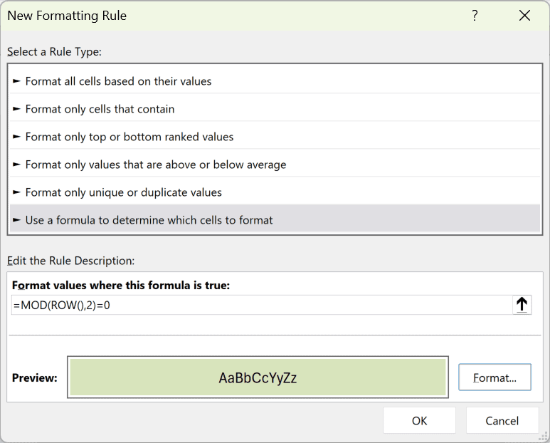
ROW() returns the row number of each cell. MOD then divides that row number by 2. Even-numbered rows return 0, so the rule is TRUE for them and the fill color gets applied.
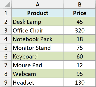
To shade odd rows instead, change the check to =MOD(ROW(),2)=1.
Example 5: Highlight Integer or Decimal Values
Here’s another conditional formatting trick built on MOD.
Below is a dataset with grocery items in column A and their weights in kilograms in column B. Some weights are whole numbers and some carry a decimal part.
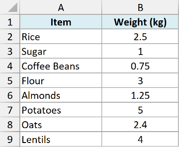
I want to highlight only the weights that have a decimal part, so the non-round values stand out.
Select the weights, go to Home, then Conditional Formatting, then New Rule, and choose the option to use a formula. Enter the formula below.
=MOD(B2,1)<>0
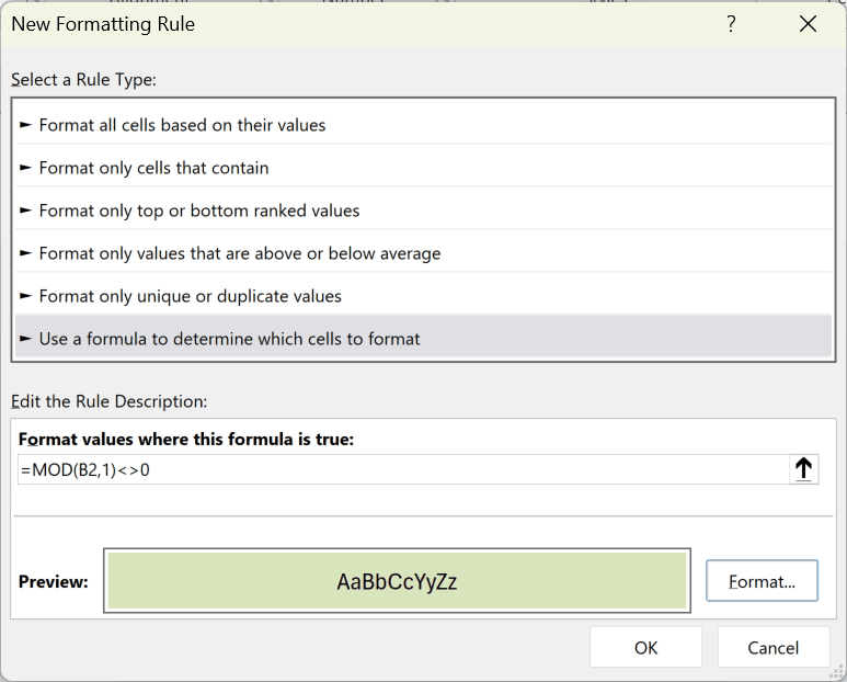
MOD(B2,1) divides each weight by 1 and returns just the fractional part. A whole number leaves 0, while a decimal leaves something other than 0, so the <>0 test is TRUE only for the decimals.
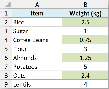
To highlight the whole numbers instead, flip the test to =MOD(B2,1)=0.
Pro Tip: Point the formula at the first cell of your selection with a relative reference (B2 here), not an absolute one like $B$2. Conditional formatting shifts that reference down the range for you.
Example 6: Sum Every Nth Row
Let’s step it up with a more useful case.
Below is a dataset with 12 days of sales, with the day in column A and the amount in column B. The data runs from row 2 to row 13.
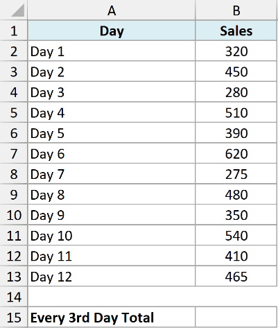
I want to add up only every 3rd day (day 3, day 6, day 9, and day 12), maybe because that’s when a promotion ran.
Here is the formula:
=SUMPRODUCT((MOD(ROW(B2:B13)-ROW(B2)+1,3)=0)*B2:B13)
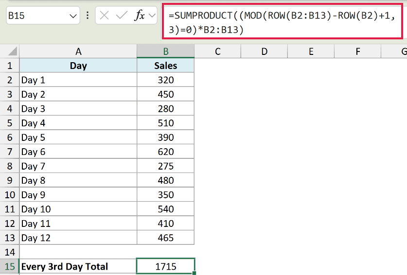
How this formula works:
ROW(B2:B13)-ROW(B2)+1numbers the rows 1 through 12, no matter where the table sits on the sheet.MOD(...,3)=0is TRUE only on positions 3, 6, 9, and 12 (the ones that divide evenly by 3).- SUMPRODUCT multiplies those TRUE/FALSE results by the sales values and adds up the matches, giving the total for every 3rd day.
Example 7: Create a Repeating Sequence
This next one is something I use for rotation and scheduling.
Below is a dataset with 9 support tickets in column A. I want to assign them to three agents in a repeating 1, 2, 3, 1, 2, 3 pattern so the work is split evenly.
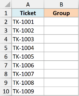
I want a group number next to each ticket that cycles through 1, 2, and 3 and then starts over.
Here is the formula:
=MOD(SEQUENCE(9,1,0),3)+1
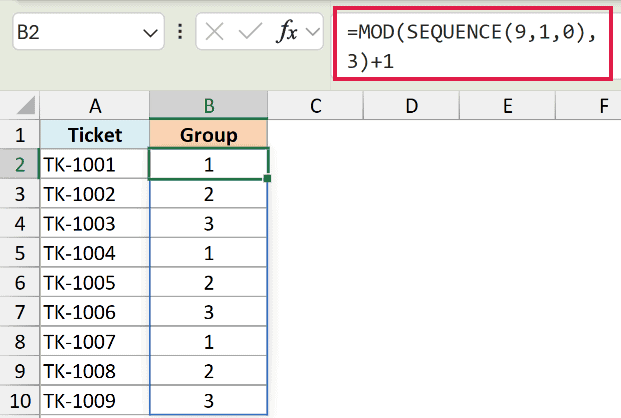
SEQUENCE(9,1,0) spills the numbers 0 through 8 down the column. MOD divides each by 3, which wraps the count into 0, 1, 2, 0, 1, 2, and so on. Adding 1 shifts that into the friendlier 1, 2, 3 range.
SEQUENCE needs Excel 365 or 2021. On older versions, put =MOD(ROW()-2,3)+1 in the first cell (row 2 here) and drag it down for the same cycle.
Pro Tip: To show names instead of numbers, wrap it in CHOOSE, like =CHOOSE(MOD(SEQUENCE(9,1,0),3)+1,"Alex","Bina","Carl"), and the three agents rotate down the list.
Example 8: Split Total Seconds into Minutes and Seconds
Let’s finish with a time example.
Below is a dataset with runner names in column A and each runner’s lap time recorded as a plain count of seconds in column B.
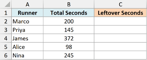
I want to pull out just the seconds portion of each time first, then build a clean minutes and seconds label.
Here is the formula for the leftover seconds:
=MOD(B2:B6,60)
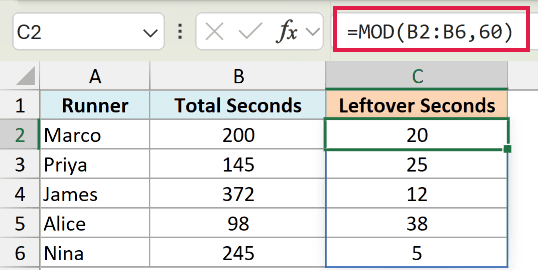
Dividing by 60 and taking the remainder gives you the seconds that don’t make up a full minute. A total of 200 seconds returns 20, because 200 is three full minutes (180 seconds) plus 20.
Now here is the formula that combines the minutes and the seconds into one label:
=INT(B2:B6/60)&":"&TEXT(MOD(B2:B6,60),"00")
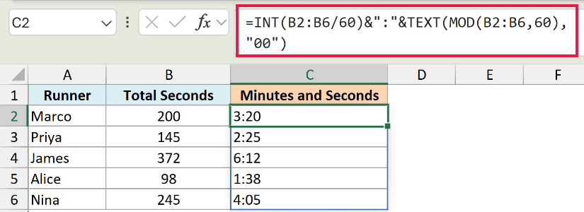
INT(B2/60) gives the whole minutes, MOD(B2,60) gives the leftover seconds, and TEXT pads the seconds to two digits. So 200 seconds reads as a clean 3:20.
Tips & Common Mistakes
- A divisor of 0 gives an error. MOD cannot divide by zero, so
=MOD(10,0)returns the #DIV/0! error. Make sure the divisor cell is never blank or zero. - The result follows the sign of the divisor, not the number. This surprises people coming from other tools.
=MOD(-3,2)returns 1 (positive, matching the divisor), while=MOD(3,-2)returns -1. - MOD and INT/QUOTIENT are a pair for nonnegative quotients. MOD gives the leftover, and INT or QUOTIENT gives the whole-number part. With a negative quotient, INT rounds down but QUOTIENT truncates toward zero; MOD follows
number-divisor*INT(number/divisor). - MOD works with decimals too.
=MOD(6.25,1)returns 0.25, which is a quick way to grab just the fractional part of a number.
That covers the MOD function, from plain remainders to the handier tricks like shading alternating rows and building repeating sequences. The core idea is always the same: divide, then keep the leftover.
Once that clicks, you’ll start noticing spots to use it in your own workbooks.
Other Excel Articles You May Also Like:
