ISOMITTED Function in Excel

The ISOMITTED function checks whether an argument was left out when a LAMBDA is called, and returns TRUE or FALSE. That’s what lets you build your own functions with optional arguments that fall back to a default value.

ISOMITTED only works inside a LAMBDA, and it checks a parameter name, not a cell. Point it at a regular cell and it returns FALSE instead of an error, so nothing warns you that it isn’t doing anything useful.

In this tutorial, I’ll show you how to use ISOMITTED to set default values, build custom functions with optional arguments in Name Manager, handle blank cells, and work with more than one optional argument.

ISOMITTED Function Syntax

Here is the syntax of the ISOMITTED function:

=ISOMITTED(argument)

• argument – the name of a LAMBDA parameter you want to check, such as tip_pct in LAMBDA(bill,[tip_pct],...).

ISOMITTED returns TRUE when that argument was left out of the call, and FALSE when a value was passed in. It looks at whether the argument was supplied, not at what the value is.

To let someone leave an argument out in the first place, put its name in square brackets in the LAMBDA, like [tip_pct]. The brackets tell Excel the argument is optional.

Optional arguments have to come after the required ones. Excel won’t accept a LAMBDA like =LAMBDA([a],b,a+b), so put the arguments people always need first.

The ISOMITTED function works in Excel for Microsoft 365 (Windows and Mac) and Excel 2024. It’s not available in Excel 2021 or earlier versions.

When to Use the ISOMITTED Function

Use this function when you need to:

• Give an optional LAMBDA argument a default value, so the function still works when that argument is skipped
• Build reusable custom functions in Name Manager with both required and optional arguments
• Tell the difference between an argument that was left out and one that was passed as empty text
• Show a clear result instead of a silent zero when an input is missing

Let me show you a few practical examples of how to use ISOMITTED.

Example 1: Set a Default Value for a Missing LAMBDA Argument

Let’s start with a simple example that shows why ISOMITTED is needed in the first place.

Below I have a list of online orders, and I want a total that adds $5 shipping whenever no shipping amount is passed to the formula. Column C shows what happens without ISOMITTED, and column D fixes it.

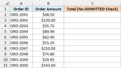
Here is the formula without the ISOMITTED check:

=LAMBDA(amount,[shipping],amount+shipping)(B2:B11)

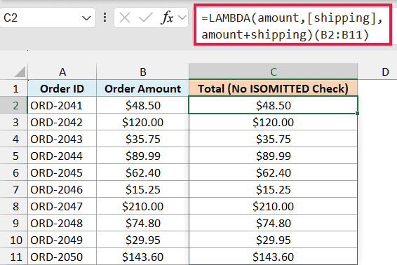
This LAMBDA takes an order amount and an optional shipping charge, and the (B2:B11) at the end runs it right away on the order amounts. If this way of calling a LAMBDA is new to you, my LAMBDA function tutorial explains it.

Since nothing is passed for shipping, Excel treats it like an empty cell, which counts as 0 in a sum.

So every total in column C is just the order amount. No shipping gets added, and there’s no error to tell you something was missing.

Here is the formula with ISOMITTED:

=LAMBDA(amount,[shipping],amount+IF(ISOMITTED(shipping),5,shipping))(B2:B11)

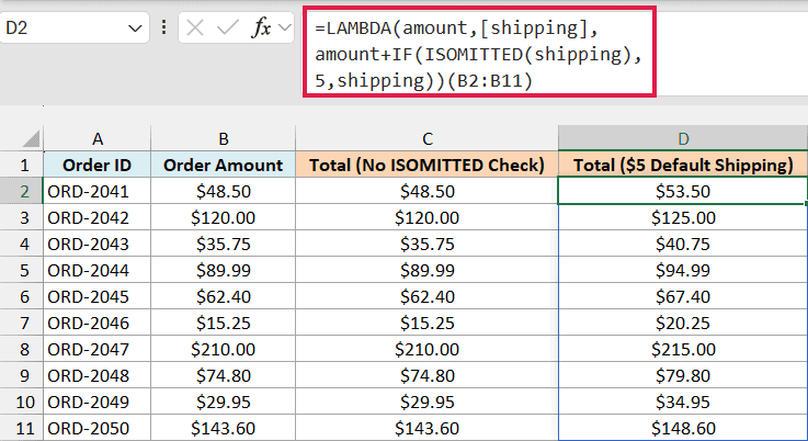
How this formula works:

• [shipping] is in square brackets, which makes it an optional argument.
• ISOMITTED(shipping) returns TRUE because the call only passes the order amounts.
• IF then uses 5 as the shipping charge. If you passed a value instead, like (B2:B11,8), ISOMITTED would return FALSE and the formula would add 8.
• Since B2:B11 is a range, the results spill into D2:D11 on their own.

Important: Without the square brackets, skipping the argument returns a #VALUE! error, so ISOMITTED never gets the chance to run.

Writing a LAMBDA straight into a cell like this is handy for testing. In practice, you’d save it as a named function so you can reuse it, which is what the next example does.

Example 2: Create a Custom Function With Optional Parameters

Now let’s save a LAMBDA with an optional argument under a name, so it works like a regular function anywhere in the workbook.

Below is a list of restaurant bills, and I want to calculate the tip at a default 15% in column C, and at 20% in column D.

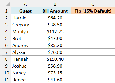
First, save the LAMBDA as a named function called TipAmount. Open Name Manager (Formulas tab > Name Manager, or Control + F3), click New, enter TipAmount as the name, and paste this formula in the Refers to field:

=LAMBDA(bill,[tip_pct],bill*IF(ISOMITTED(tip_pct),15%,tip_pct))

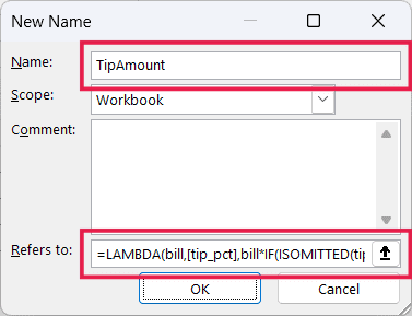
Click OK, and TipAmount now works like any other function in this workbook. If you’ve never saved a LAMBDA in Name Manager before, my LAMBDA tutorial (linked in Example 1) walks through it step by step.

Here is the formula for the 15% tip:

=TipAmount(B2:B11)

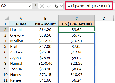
The formula only passes the bills, so tip_pct is left out. ISOMITTED(tip_pct) returns TRUE, and the function multiplies each bill by 15%.

Here is the formula for the 20% tip:

=TipAmount(B2:B11,20%)

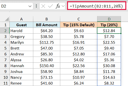
This time tip_pct is supplied, so ISOMITTED returns FALSE and the function uses 20% instead of the default.

That’s the whole idea of an optional argument. The person using TipAmount only adds the second argument when they want something other than the default, the same way you can skip the last argument in many of Excel’s own functions.

Example 3: Handle Blank Cells (ISOMITTED Returns FALSE)

Here’s a catch you’ll run into once you start feeding cell ranges into a function like TipAmount.

Below is a list of bills where a few guests picked their own tip in the Custom Tip column, and I want everyone else to get the 15% default. Column D uses TipAmount from Example 2, and column E fixes the problem it runs into.

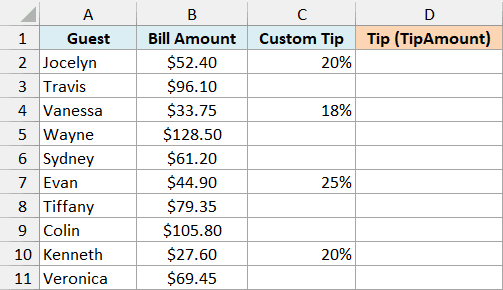
Here is the formula using TipAmount:

=TipAmount(B2:B11,C2:C11)

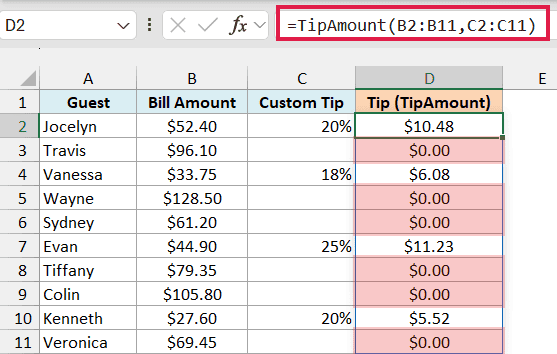
The rows with a custom tip come out right, but every row with a blank Custom Tip shows $0.00.

That’s because you passed C2:C11, blank cells and all, so the argument was never left out. ISOMITTED returns FALSE for the blank rows too, and the bill gets multiplied by an empty cell, which counts as 0.

To treat a blank cell the same as a missing argument, check whether the value is empty instead. Save this updated LAMBDA in Name Manager with the name TipAmountFix:

=LAMBDA(bill,[tip_pct],bill*IF(tip_pct="",15%,tip_pct))

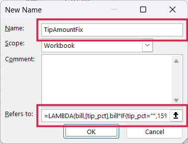
Here is the formula using TipAmountFix:

=TipAmountFix(B2:B11,C2:C11)

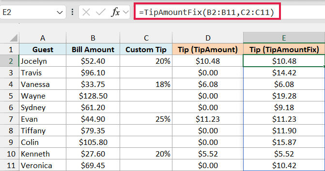
Now the blank rows get the 15% default, and the custom tips still go through. The check tip_pct="" is TRUE for a blank cell, and it’s also TRUE when the argument is left out, because a missing argument behaves like an empty cell.

So this one check covers both cases, and calling TipAmountFix with no second argument still gives the 15% tip.

Important: You may see IF(OR(ISOMITTED(tip_pct),tip_pct=""),15%,tip_pct) suggested for this. With a range, OR returns one TRUE or FALSE for the whole range, so every row gets 15% and the custom tips are ignored.

Example 4: Tell an Omitted Argument Apart From Empty Text

If checking for an empty value covers both cases, you might wonder why you’d need ISOMITTED at all. This example shows where it matters.

Below I have product categories and item numbers, and I want to build product codes with a hyphen by default in column C, and codes with no separator in column D.

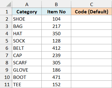
Save this LAMBDA in Name Manager with the name MakeCode:

=LAMBDA(category,num,[sep],category&IF(ISOMITTED(sep),"-",sep)&num)

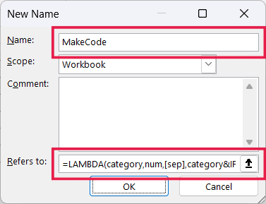
Here is the formula that uses the default separator:

=MakeCode(A2:A11,B2:B11)

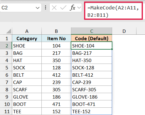
The separator is left out, so ISOMITTED(sep) returns TRUE and the function puts a hyphen between the category and the number. That gives codes like SHOE-104.

Here is the formula that passes empty text as the separator:

=MakeCode(A2:A11,B2:B11,"")

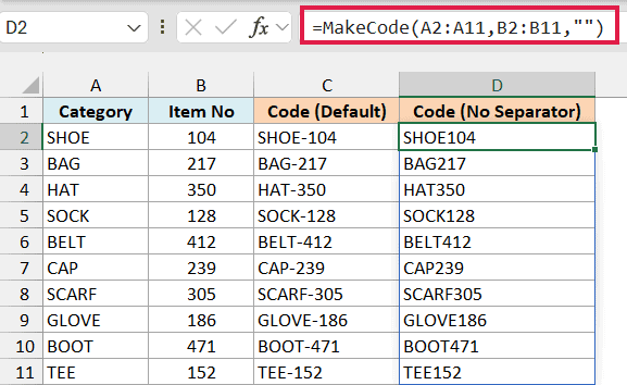
This time "" is supplied, so ISOMITTED returns FALSE and the function joins the two parts with nothing in between, giving SHOE104.

If MakeCode checked sep="" instead of using ISOMITTED, it couldn’t tell these two calls apart. Both would return SHOE-104, and there would be no way to ask for a code without a separator.

Example 5: Use Multiple Optional Arguments (and Skip One)

Let’s step it up with a function that has two optional arguments, where you only want to change the second one.

Below is a list of road trips with the distance in miles, and I want to estimate the fuel cost in column C using a default of 25 miles per gallon and $3.50 gas. In column D, I want the same estimate with $4 gas.

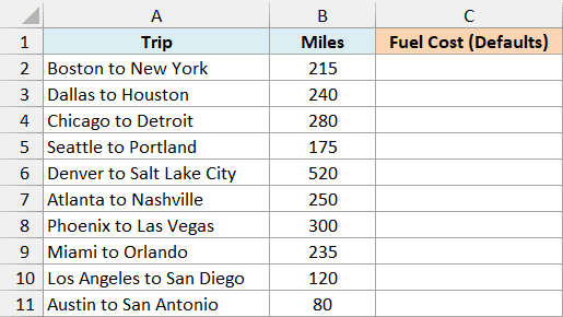
Save this LAMBDA in Name Manager with the name FuelCost:

=LAMBDA(miles,[mpg],[price],LET(m,IF(ISOMITTED(mpg),25,mpg),p,IF(ISOMITTED(price),3.5,price),miles/m*p))

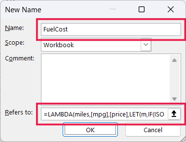
How this function works:

• [mpg] and [price] are both optional, and each gets its own ISOMITTED check. If mpg is left out it becomes 25, and if price is left out it becomes 3.5.
• LET saves the final mileage as m and the final gas price as p, which keeps the last part, miles/m*p, easy to read. My LET function guide covers how LET works.

Here is the formula that uses both defaults:

=FuelCost(B2:B11)

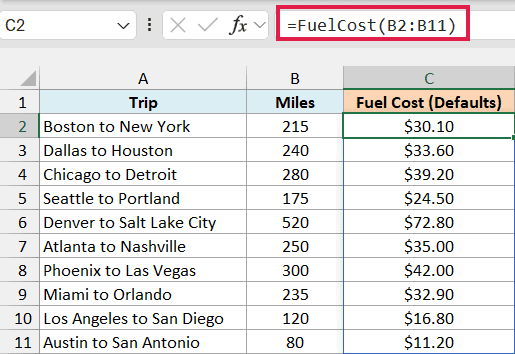
Both optional arguments are left out, so the function divides the miles by 25 and multiplies by $3.50. For the 280-mile Chicago to Detroit trip, that’s $39.20.

Here is the formula that keeps the default mileage but uses $4 gas:

=FuelCost(B2:B11,,4)

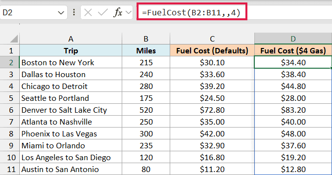
The two commas leave an empty slot for mpg, so ISOMITTED(mpg) returns TRUE and the function still uses 25. The price is supplied as 4, so the Chicago to Detroit trip now costs $44.80.

So that’s how ISOMITTED works. It’s small, but it’s what turns a LAMBDA into a proper custom function with optional arguments and sensible defaults.

Just remember that it only knows whether an argument was left out. When blank cells should also get the default, check for an empty value as shown in Example 3.

I hope you found this tutorial helpful.

List of All Excel Functions

Other Excel Articles You May Also Like:

• IS Functions in Excel
• How to Create Named Ranges in Excel
• ISBLANK Function in Excel
• 20 Advanced Excel Functions and Formulas (for Excel Pros)