
If you have a stacked column or bar chart and you want to show the total on top of each stack, you’ll notice Excel doesn’t give you a direct option for it.
The chart can happily label each segment’s value, but the one number people actually look for, the total of the stack, is missing. And this is because the chart is built only from the segment values, so there’s no total in it to label.
But nothing to worry about. It’s easy to do once you know the trick, and I’ll show you two ways to get the total onto your chart.
The first uses a hidden line series and works on stacked column charts. The second uses Value From Cells and works on stacked columns and horizontal bars.
Setting Up the Data
Before we touch the chart, let’s get the data ready. Both methods need a Total column sitting next to your category values.
Below I have monthly sales split across two product lines, Laptops and Phones, for January to April.
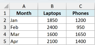
Add one more column called Total that adds the two segments together for every row. Enter this in D2 and copy it down to D5:
=SUM(B2:C2)
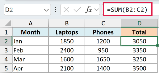
Now you have a Total value for each month, which both methods below will use.
Pro Tip: On Excel 365 or Excel 2021, enter =B2:B5+C2:C5 once in D2 and the totals spill down the column on their own, so there’s nothing to copy. On older versions, stick with the SUM formula above.
Method 1: Add the Total as an Invisible Line (Stacked Columns)
This is the method I reach for on a stacked column chart. You add the Total as an extra series, turn that series into a line, switch on its data labels, and then hide the line.
Working with a horizontal bar chart instead? Go straight to Method 2.
A line series and horizontal bars sit on axes that run in different directions, so the labels never line up and this trick can’t work there.
On a stacked column chart, the labels belong to the Total line, so they sit at the top of each column and update when your numbers change. Let me walk you through it.
We’re using the same monthly sales data, with the Total column now in column D.
Here are the steps to add total labels using a hidden line series:
- Select your full data range, including the Total column (here that’s A1:D5).
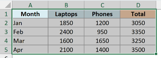
- Go to the Insert tab, click the column chart icon in the Charts group, and pick Stacked Column.
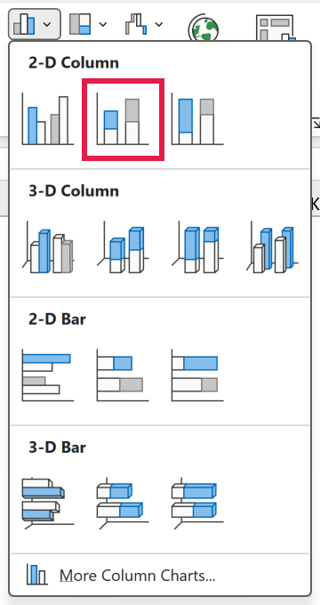
At this point the Total is stacked on top of your other segments, which looks wrong. We fix that in the next step by turning it into a line.
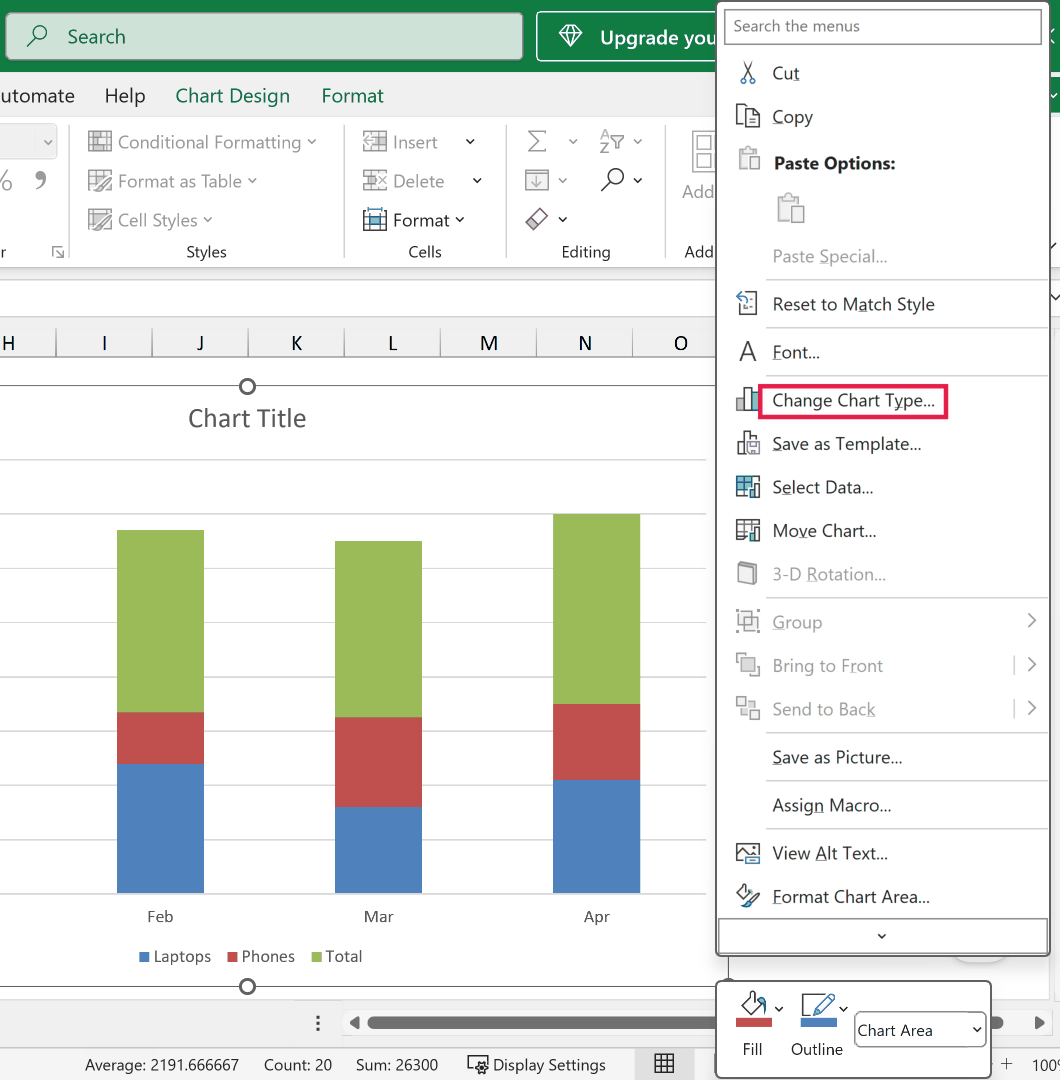
- Right-click anywhere on the chart and choose Change Chart Type.
- In the dialog box, select Combo on the left. Leave Laptops and Phones as Stacked Column, change the Total series to Line, make sure its Secondary Axis box is unticked, and click OK.
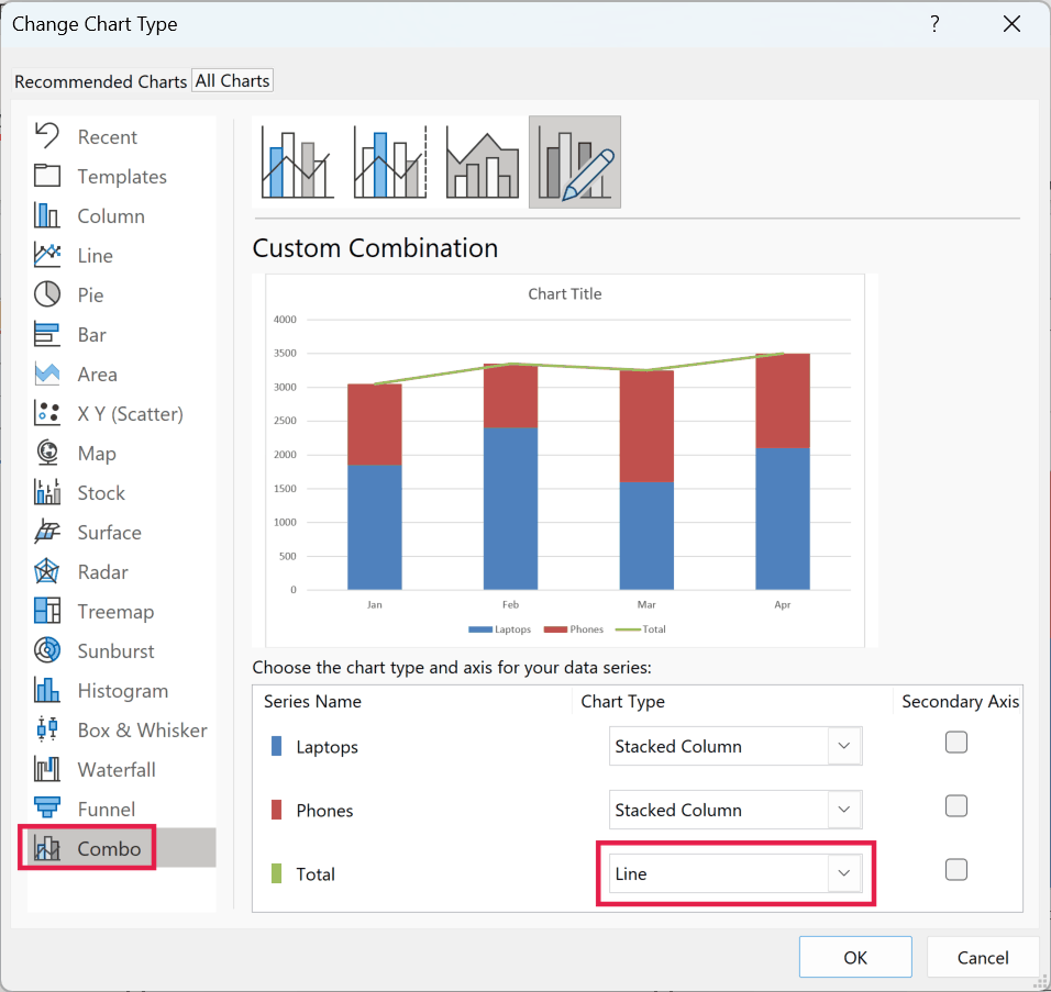
You’ll now see a line running across the top of your columns. That line is the total, and it’s exactly what we’ll label.
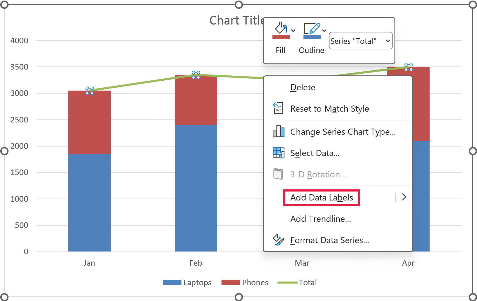
- Right-click the Total line and choose Add Data Labels.
- Right-click the Total line again and choose Format Data Series. In the pane on the right, open the paint-bucket (Fill & Line) section, select No line, and the line disappears while the labels stay put.
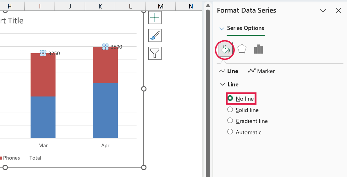
The totals now show at the top of each stacked column. Excel places them to the right of each point by default, so they look a little off-center, and the next step fixes that.
- Click any total label to select all of them, right-click, and choose Format Data Labels. Under Label Position, select Above.
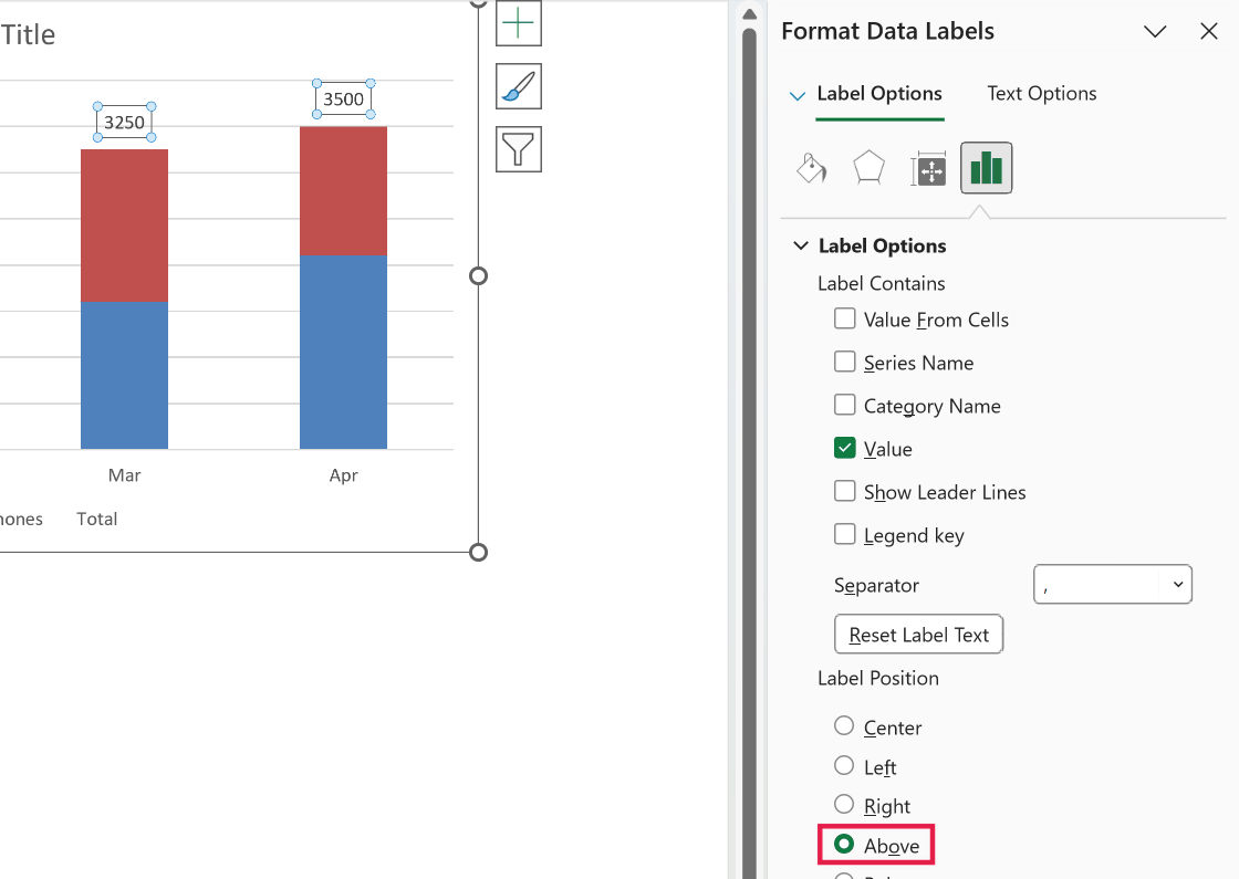
That’s it. You now have clean total labels sitting above every column, and they’ll update on their own whenever your sales numbers change.
If the Total still shows in the legend, click the legend once, click the Total entry to select just that item, and press Delete to remove it.
Pro Tip: To format the totals, select the total labels, open Format Data Labels, and under Number set a format like #,##0 or a currency format. The labels then read the same way as your data.
Method 2: Use Value From Cells (Columns and Bars)
Here’s another way to do this that skips the line series entirely. Instead, you add a plain set of data labels to one of the existing segments and tell Excel to pull the label text from your Total column.
This is also the method to use on a horizontal stacked bar chart, since it doesn’t need a line series at all.
The trade-off is that the labels are tied to a segment rather than floating above the stack, so you’ll usually want to reposition them.
Let’s suppose you have a stacked column chart (or stacked bar chart) built from A1:C5, so just the months, Laptops, and Phones. Leave the Total column out of the chart, or it stacks on top as an extra segment.
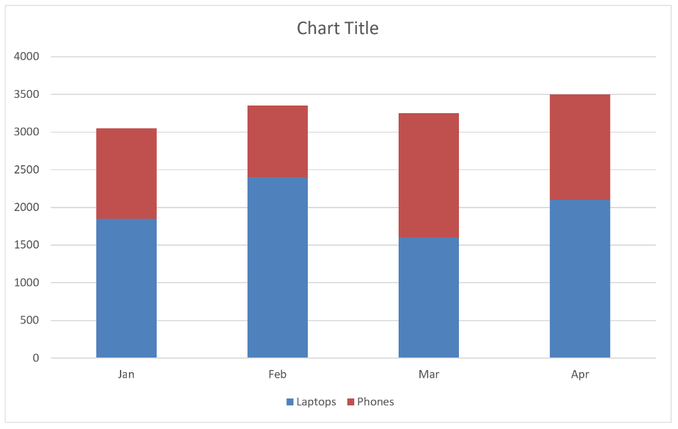
Here are the steps to label the totals using Value From Cells:
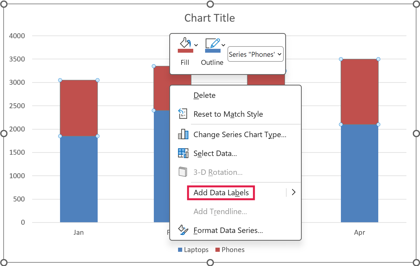
- Right-click the top segment of the stack (Phones here, or the segment at the right end on a bar chart) and choose Add Data Labels.
- Right-click any of the new labels and choose Format Data Labels to open the pane on the right.
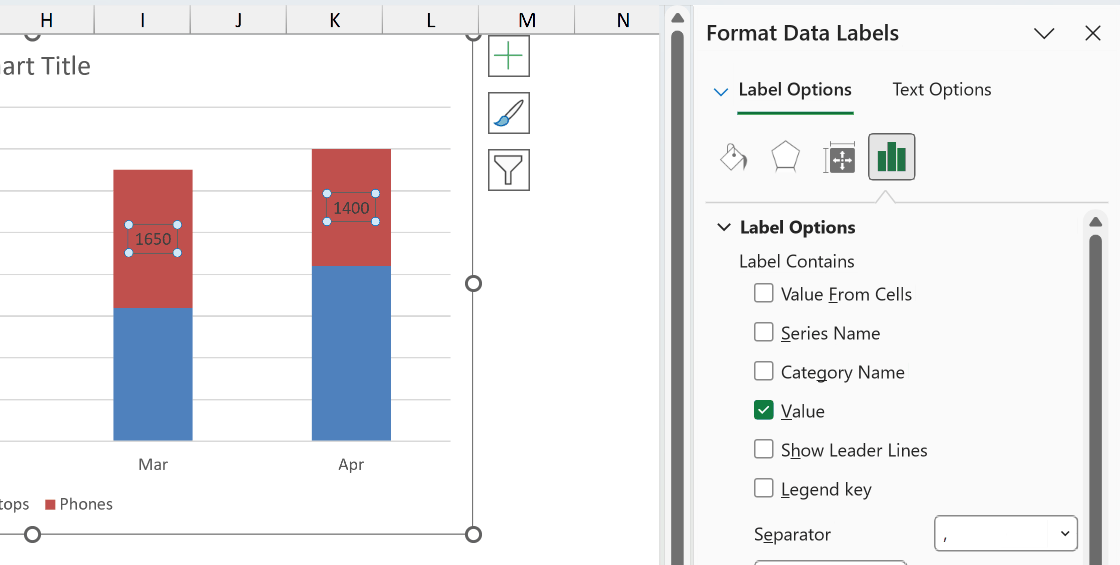
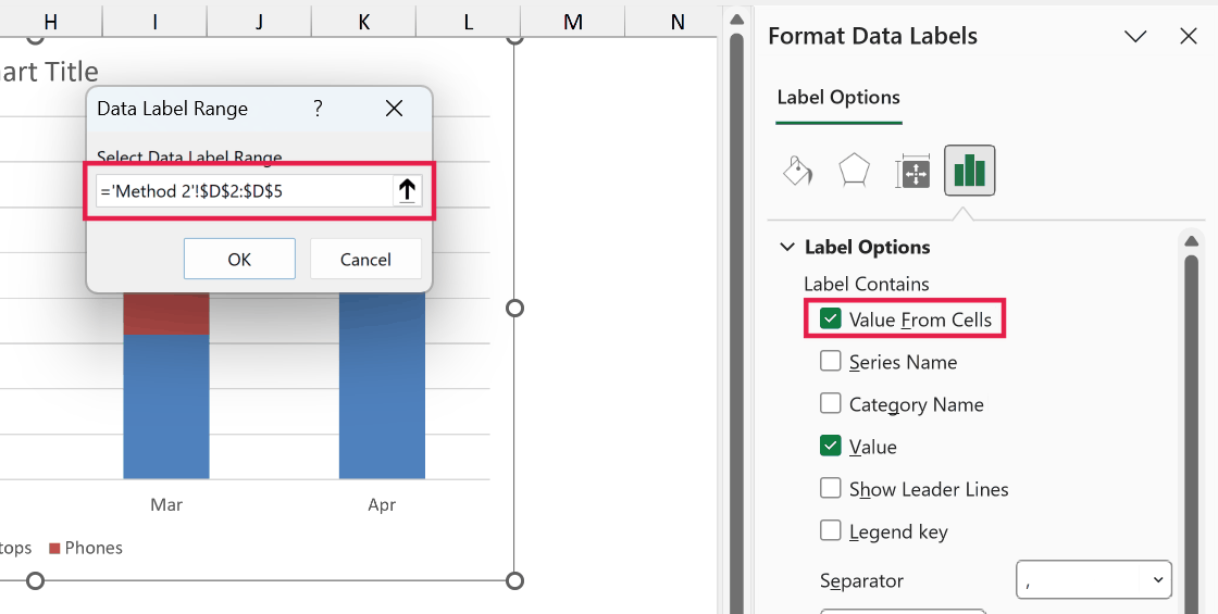
- In the pane, under Label Options, tick Value From Cells. In the box that pops up, select your Total column range (D2:D5 here) and click OK.
- Still in the pane, untick Value so the labels show only the total, not the segment’s own number.
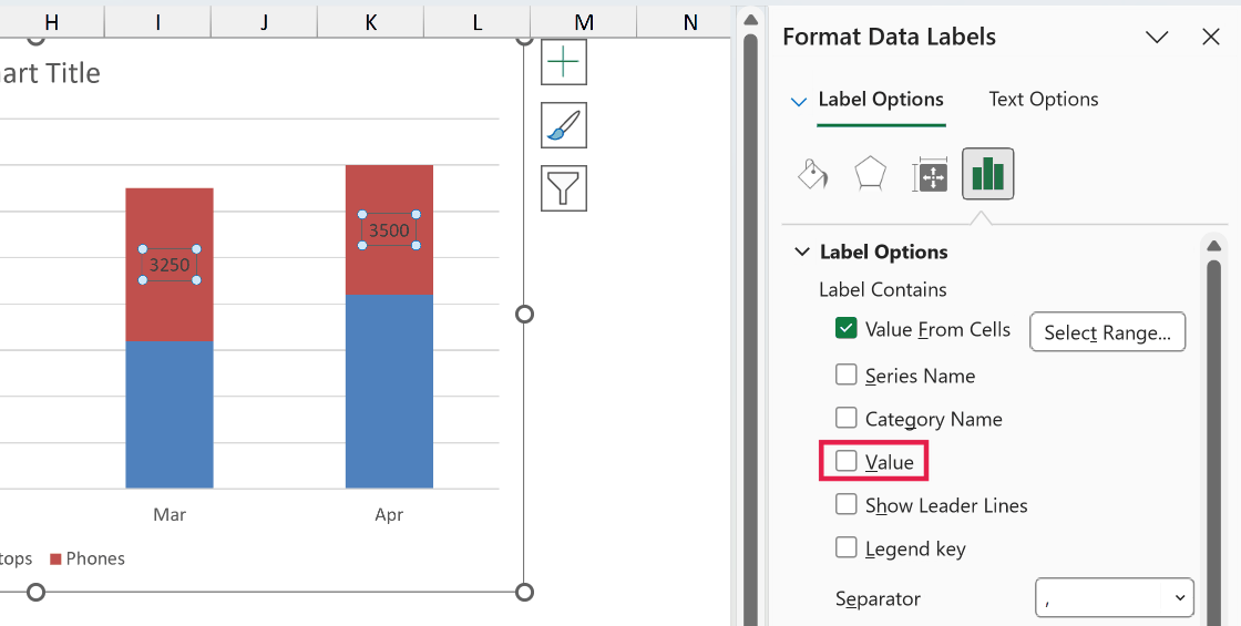
Your totals now appear on the chart, pulled straight from the Total column. The only thing left is to move them where you want.
- With the labels still selected, in the same pane set Label Position to Inside End.
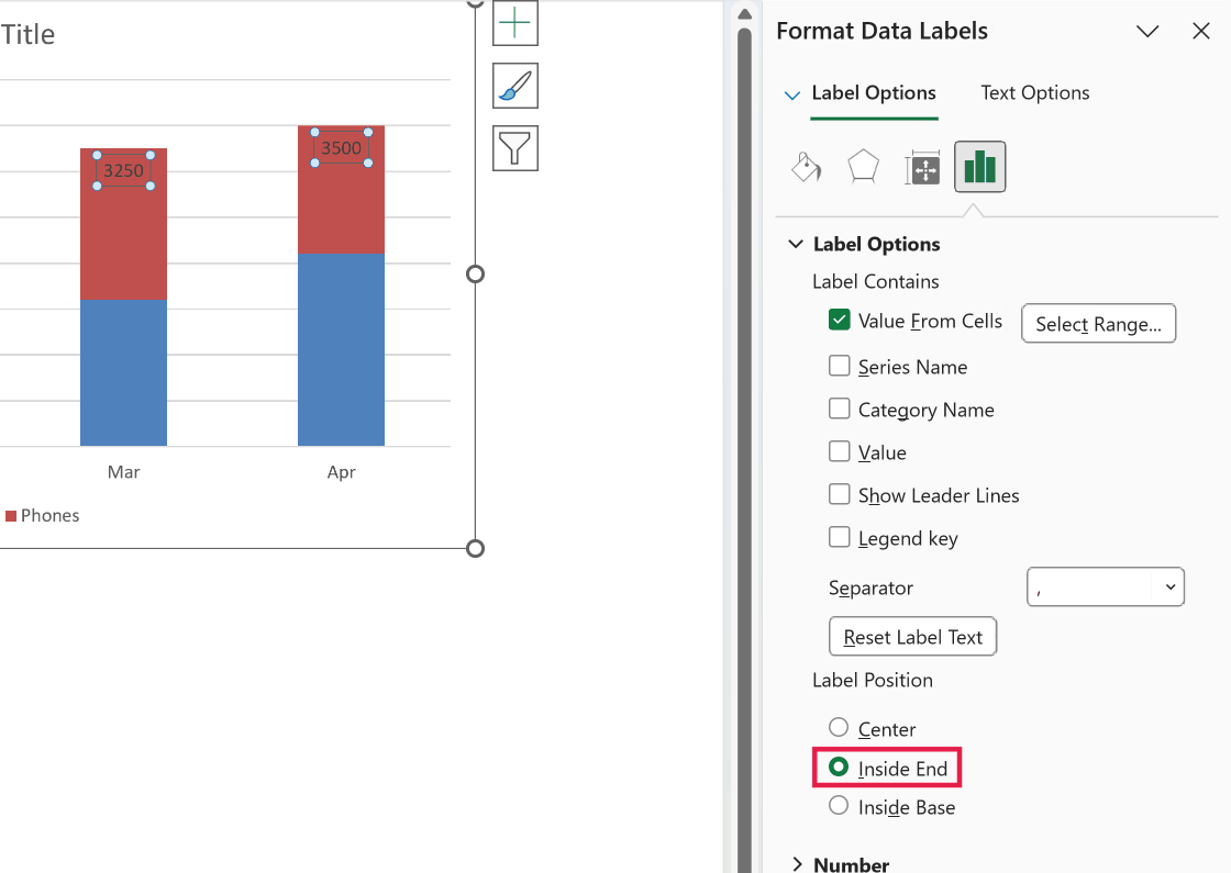
On a stacked column, Inside End puts the total just inside the top of the stack. On a horizontal bar, it puts the total just inside the right end of the bar.
Since the label sits inside the segment, it’s worth making it bold or white so nobody reads it as the Phones number.
Pro Tip: If the top segment is short, a long total label can overflow into the segment next to it. Shrinking the label font or switching to a shorter number format usually clears it up.
This method is quick, but remember the labels are tied to a segment. On a stacked column chart, Method 1 gives you a cleaner result with the totals floating above the columns.
Things to Keep in Mind
- The total labels stay accurate only if your Total column is correct. Always build it with a formula that adds the segments so it updates when the data changes, rather than typing numbers in by hand.
- In Method 1, the Total series briefly distorts your chart before you turn it into a line. Don’t panic when the total stacks on top of your columns. It looks right again the moment you switch it to a line and pick No line.
- Method 1 only works on stacked column charts. On a horizontal stacked bar chart, use Method 2.
- Value From Cells needs Excel 2013 or later, and it’s in all Microsoft 365 versions. If you’re on an older build and don’t see the option, use the line series method instead.
- On Excel 2010 or older, the Change Chart Type dialog has no Combo option. In Method 1, replace steps 3 and 4 by right-clicking the Total series, choosing Change Series Chart Type, and picking Line.
- If you add or remove months later, copy the SUM formula down to the new rows (or extend the ranges in the spill formula) and extend the chart’s data range. In Method 2, also check that the Value From Cells range still covers all your rows.
In this article I showed you two ways to add total values to a stacked chart, using a hidden line series and using Value From Cells.
The line series method is for stacked columns, and Value From Cells works on stacked columns and horizontal bars.
I hope you found this article helpful.
Other Excel Articles You May Also Like: