

If you want to add up numbers in Excel, the SUM function is what you reach for. It doesn’t matter if they sit in one column, are scattered across a few cells, or spread over several sheets.
You give it the numbers to add, and it returns a single total. SUM also works seamlessly inside dynamic array formulas like =SUM(FILTER(...)), so you can total just the rows that meet a condition.
In this article I’ll show you how to use SUM in Excel, starting with a plain range total and building up to non-adjacent cells, a running total, 3D references across sheets, and a conditional total.
SUM Function Syntax
Here is the syntax of the SUM function:
=SUM(number1, [number2], ...)
- number1 – the first value you want to add. This can be a number like 25, a single cell reference like B2, or a whole range like B2:B8. This one is required.
- [number2], … – optional extra values or ranges to add. You can keep adding these, up to 255 of them in a single formula.
SUM works in Excel for Microsoft 365, Excel 2024, 2021, 2019, 2016, and older versions, plus Excel on the web and Excel for Mac. It’s about as universal as a function gets.
When to Use the SUM Function
Use the SUM function when you need to:
- Add up a column or row of numbers to get a total
- Total a few specific cells that aren’t next to each other
- Build a running (cumulative) total down a column
- Roll up the same cell across several identical sheets
If you only want to add numbers that meet a condition (like sales for one region), that’s a job for SUMIF or SUMIFS instead. I’ll point you there where it fits.
Let me show you a few practical examples of how SUM works.
Example 1: Add Up a Range of Numbers
Let’s start with the most common use, adding up a single range.
Below I have the amounts raised each day at a school bake sale, with the day in column A and the amount in column B.
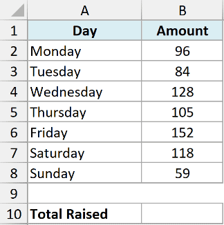
I want the total raised across all seven days in one cell.
Here is the formula:
=SUM(B2:B8)
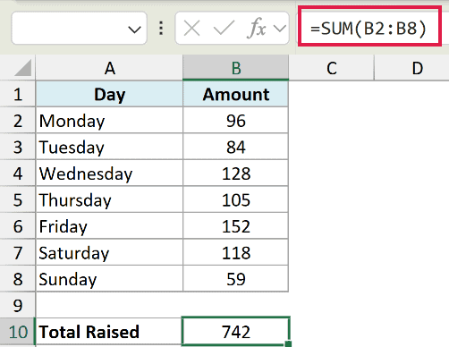
This gives me 742. SUM looks at every cell from B2 to B8, adds the numbers together, and returns the total. If you change any daily amount, the total updates on its own.
Pro Tip: Instead of typing the formula, select the cell right below your numbers and press Alt + = (the AutoSum shortcut). Excel writes the SUM formula and guesses the range for you. Just check the range and press Enter.
Example 2: Sum Cells That Aren’t Next to Each Other
Here’s a common one that trips people up. Sometimes the cells you want to add aren’t in one tidy block.
Below is a small project cost sheet. Column A has the cost item, column B has the type (Labor or Material), and column C has the amount. The labor rows sit in two separate groups.
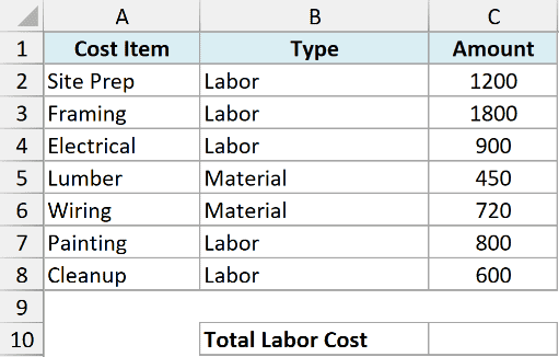
I want to add up only the labor costs, which live in C2:C4 and C7:C8.
Here is the formula:
=SUM(C2:C4, C7:C8)
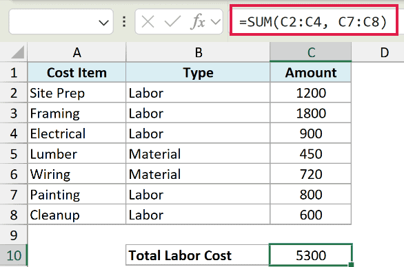
This returns 5300. You just list each range or cell inside SUM, separated by commas. Excel adds all of them together as if they were one group.
You can mix ranges and single cells freely, like =SUM(C2:C4, C7, C10). Each item you separate with a comma becomes another thing to add.
Example 3: Create a Running Total With SUM
A running total (also called a cumulative sum) shows how a number builds up row by row. The trick is an anchored reference that grows as you copy the formula down.
Below I have monthly savings, with the month in column A and the amount saved in column B. I want a running total in column C, so each row shows the total saved up to that point.
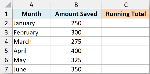
I’ll put this formula in C2 and copy it down the column.
Here is the formula:
=SUM($B$2:B2)
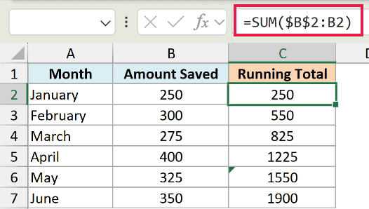
How this formula works:
- $B$2 is an absolute reference (locked with the $ signs), so the start of the range never moves as you copy down.
- B2 is a relative reference, so it shifts to B3, B4, and so on as the formula moves down.
- The result is a range that keeps stretching. In row 2 it sums B2:B2, in row 3 it sums B2:B3, and so on down the column.
So the mixed anchor is the whole point here. If you want more ways to do this, I have a full guide on the running total in Excel.
Example 4: Sum the Same Cell Across Multiple Sheets
SUM can also add the same cell across several sheets at once using what’s called a 3D reference. This is handy when each sheet has the exact same layout.
Say I have three sheets named Downtown, Airport, and Mall, one per store location. Each sheet has monthly revenue laid out the same way, and the yearly total for that store sits in cell B14.
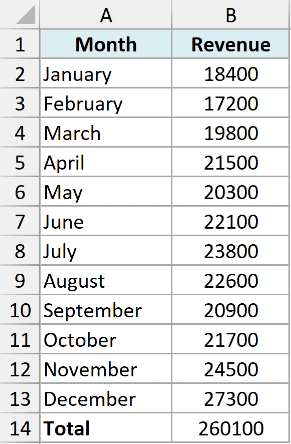
On a summary sheet, I want the combined yearly revenue from all three stores.
Here is the formula:
=SUM(Downtown:Mall!B14)

The part before the exclamation mark, Downtown:Mall, means “every sheet from Downtown through Mall in the tab order.” SUM then adds up cell B14 from each of those sheets.
The easy way to write this is to type =SUM(, click the first sheet tab, hold Shift, click the last sheet tab, then click the cell and press Enter. Excel builds the 3D reference for you.
Pro Tip: 3D references only work with a handful of functions like SUM, AVERAGE, and COUNT. SUMIF and SUMIFS can’t use them, so SUM is your go-to for a quick roll-up across identical sheets. Full walkthrough here: how to sum across multiple sheets.
Example 5: SUM Ignores Text and Blank Cells
A lot of people worry that a stray word or an empty cell will break their SUM. It won’t, and this example shows why.
Below is a reading log with the day in column A and pages read in column B. On some days there’s a number, on others it says “Rest day,” and one cell is just blank.
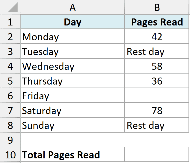
I want the total pages read, without cleaning up the text or blanks first.
Here is the formula:
=SUM(B2:B8)
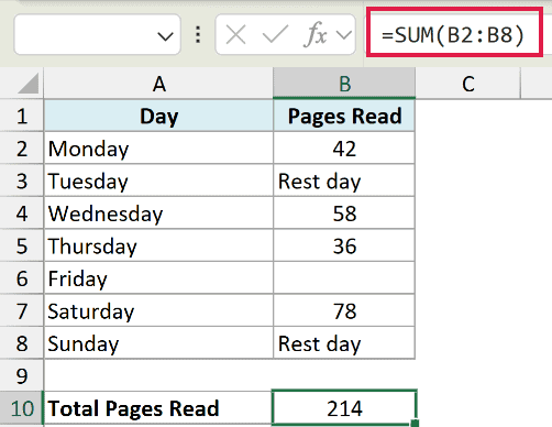
This returns 214. When SUM looks at a range, it quietly skips anything that isn’t a number, so the “Rest day” text and the empty cell are ignored. Only the real numbers get added.
This is why SUM is safer than adding cells with plus signs. A formula like =B2+B3+B4 would throw a #VALUE! error the moment it hits that “Rest day” text.
Example 6: Sum an Entire Column in Excel
If your data keeps growing, you can point SUM at a whole column instead of a fixed range. New rows get included automatically.
Below is an order log that gets new rows added all the time. The order ID is in column A and the order value is in column B, with a header row on top.
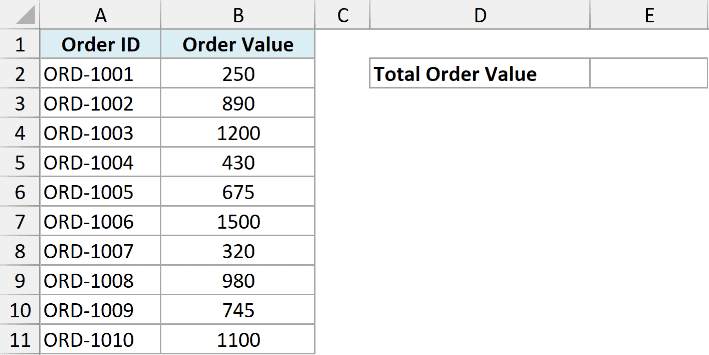
I want a total order value that updates on its own whenever a new order is added.
Here is the formula:
=SUM(B:B)
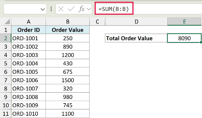
B:B means the entire column B. SUM adds every number in it, and since it ignores text, the “Order Value” header doesn’t cause a problem. Add a new order at the bottom and the total picks it up right away.
Just make sure the SUM formula itself sits outside column B (in a different column), or you’ll create a circular reference. For more options, see my guide on how to sum a column in Excel.
Example 7: Sum Only the Values That Meet a Condition
Now for the modern one. On Excel 365 or 2021, you can wrap SUM around the FILTER function to total only the rows that meet a condition, all in one formula.
Below is a sales table with the product in column A, the category in column B, and the amount in column C. I want the total sales for just the “Coffee” category.
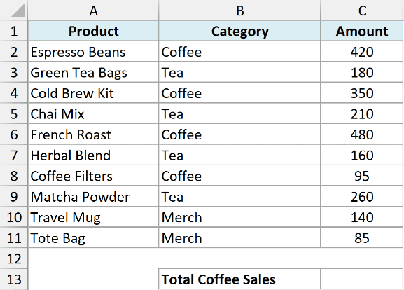
I want a single number: the sum of every Coffee row’s amount.
Here is the formula:
=SUM(FILTER(C2:C11, B2:B11="Coffee"))
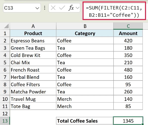
Here is how it works:
- FILTER(C2:C11, B2:B11=”Coffee”) pulls out just the amounts where the category is Coffee, returning them as an array.
- SUM then adds up that filtered array and collapses it into a single total.
This is a good way to see how SUM composes with dynamic array functions. FILTER produces the array, and SUM reduces it to one value.
Pro Tip: For a plain conditional total like this, SUMIF is usually simpler and works in every Excel version: =SUMIF(B2:B11,”Coffee”,C2:C11). Reach for SUM(FILTER(…)) when you also want the filtered rows spilled out somewhere, or when the condition is more complex.
Tips and Common Mistakes to Keep in Mind
A few things that catch people out with the SUM function:
- Numbers stored as text won’t add. If a “number” is actually text (often left-aligned, sometimes with a little green triangle in the corner), SUM skips it and your total comes up short. Select those cells, click the warning icon, and choose “Convert to Number” to fix it.
- SUM ignores text and blanks, but not errors. A word or empty cell in the range is simply skipped. But if any cell holds an error like #N/A or #DIV/0!, SUM returns that same error. Clean up the error first.
- Use SUMIF or SUMIFS for conditions. SUM adds everything in the range. To add only the rows that meet a condition, use SUMIF for one condition or SUMIFS for several.
- Watch for circular references. If the SUM formula is inside the range it’s adding, Excel flags a circular reference. Keep the total cell outside the range.
- AutoSum is the fast way in. For a quick column or row total, select the cell next to your numbers and press Alt + = to use AutoSum rather than typing the formula out.
Wrapping Up
SUM is the function you’ll use more than almost any other. Start with a simple range total, then lean on non-adjacent ranges, a mixed anchor for running totals, and 3D references when you need to roll up across sheets.
And when you need to add only certain rows, remember that SUMIF, SUMIFS, and SUM wrapped around FILTER are all there for you.
I hope you found this tutorial helpful. Let me know in the comments if you have a SUM scenario you’re stuck on.
Other Excel Articles You May Also Like:
