

Say you have twelve monthly sheets that all look the same, and you want one total that pulls the same cell from each sheet.
The manual way is to type out =Jan!B5+Feb!B5+Mar!B5 and keep going… for nine more months.
There is a much better way. It is called a 3D reference, and it lets you point one formula at the same cell across a whole run of sheets at once.
Instead of that growing chain of pluses, you write =SUM(Jan:Dec!B5) and you are done.
In this article, I’ll show you what a 3D reference is, how to build one by clicking through your sheet tabs, which functions support it, and a few things to watch out for.
What Is a 3D Reference in Excel?
A 3D reference is a single reference that points to the same cell or range across several sheets that sit next to each other.
Say you have three sheets named Jan, Feb, and Mar, and each one has its monthly total sitting in cell B5. A 3D reference lets you total that same B5 across all three sheets in one go.
Here is what such a formula looks like:
=SUM(Jan:Mar!B5)
The Jan:Mar part is the range of sheets, from the first sheet to the last. The !B5 part is the cell you want to pull from each of those sheets.
So instead of writing =Jan!B5+Feb!B5+Mar!B5, you let Excel walk through every sheet from Jan to Mar and grab B5 from each one.
This works best when your sheets share an identical layout. If B5 means the monthly total on the Jan sheet, it needs to mean the same thing on Feb and Mar for the result to make sense.
How to Build a 3D Reference by Clicking
You do not have to type the sheet names by hand. The easier way is to let Excel build the reference as you click through the sheet tabs.
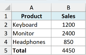
Let’s suppose you have a workbook with three sheets named Jan, Feb, and Mar. Each sheet lists the same products down column A and their sales in column B, and the total sits in B5.
You want a summary cell on a separate sheet that adds up B5 across all three months.
Here are the steps to build the 3D reference by clicking:
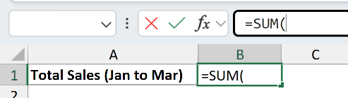
- Click the cell where you want the result, then type =SUM( to start the formula.
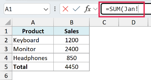
- Click the Jan sheet tab (this is your first sheet).
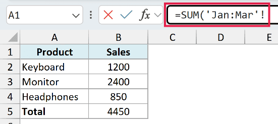
- Hold the Shift key and click the Mar sheet tab (this is your last sheet). Excel now has the whole Jan to Mar span sitting in the formula.
- Click cell B5 on the sheet that is showing.
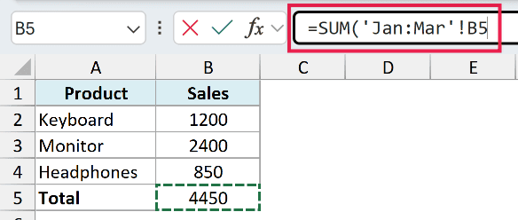
- Press Enter.
Excel closes the formula for you and shows the total of B5 from all three sheets. The finished formula reads =SUM(Jan:Mar!B5).
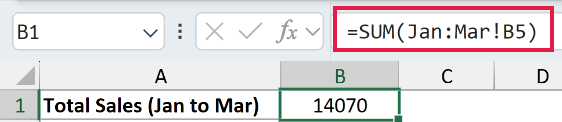
The sheets look grouped while you are building the formula, but that grouping goes away the moment you press Enter. You are not left in group mode, so you will not accidentally type into all three sheets at once.
You can also select a range instead of a single cell. If you click and drag over B2:B4 in step 4, you get =SUM(Jan:Mar!B2:B4), which adds every one of those cells across the three sheets.
Leave B5 out of that range. It already holds the total for the sheet, so including it would count every number a second time and hand you double the answer.
Once you know the pattern, you can also just type the whole reference yourself. Click the summary cell and enter =SUM(Jan:Mar!B5) directly. Clicking is only the easy way to get the sheet names right without a typo.
If you plan to reuse the same span in several formulas, you can save it as a name. Go to Formulas and click Define Name, then build the reference in the Refers to box by clicking the tabs the same way.
If adding up a single cell across every sheet is really all you need, I go deeper on that exact case in my guide on how to sum across multiple sheets in Excel.
Pro Tip: If a sheet name has a space in it, like “Q1 Sales”, Excel wraps the sheet range in single quotes, so the formula looks like ='Q1 Sales:Q3 Sales'!B5. The single quotes go around the whole sheet range, not each name.
Which Functions Support 3D References
Not every function can use a 3D reference. The ones that work are the math and statistical functions that take a simple set of values, plus the two stacking functions.
Here are the functions that support 3D references:
- SUM to add the values
- AVERAGE and AVERAGEA to get the average
- COUNT and COUNTA to count cells
- MAX and MAXA to find the highest value
- MIN and MINA to find the lowest value
- PRODUCT to multiply the values
- STDEV.S, STDEV.P, STDEVA, and STDEVPA for standard deviation
- VAR.S, VAR.P, VARA, and VARPA for variance
- VSTACK and HSTACK to pile the ranges from every sheet into one array
The older STDEV, STDEVP, VAR, and VARP names work with 3D references too, so an older workbook will not break.
Let’s look at one of these in action. We are back to the same three sheets (Jan, Feb, and Mar), each holding its monthly total in cell B5, and this time we want the average of that B5 figure across all three months.
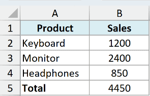
Here is the formula:
=AVERAGE(Jan:Mar!B5)
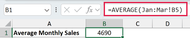
This walks through Jan, Feb, and Mar, picks up B5 from each, and returns the average of those three numbers.
Now for the part that trips people up. The lookup and conditional functions do not support 3D references.
That means XLOOKUP, VLOOKUP, INDEX, MATCH, SUMIF, SUMIFS, COUNTIF, and COUNTIFS will not let you point at a Jan:Mar! style range.
SUBTOTAL and AGGREGATE are out as well. Both return a #VALUE! error if you feed them a sheet span, which surprises a lot of people who reach for SUBTOTAL first.
How to Do a Conditional Total Across Sheets with VSTACK
So what do you do when you actually need a conditional total across sheets? This is where VSTACK earns its keep.
VSTACK does accept a 3D reference, and it stacks the range from every sheet in the span into one tall array. Once the data is in a single array, the conditional functions can work on it.
Let’s stay with the same Jan, Feb, and Mar sheets, where each one lists products in A2:A4 and their sales in B2:B4.
Start by stacking all three months into one list:
=VSTACK(Jan:Mar!A2:B4)
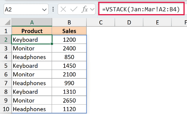
That gives you all nine rows in one spilled range, with the products in the first column and the sales in the second.
Now wrap it in FILTER and SUM to get the total for one product across all three months:
=SUM(FILTER(VSTACK(Jan:Mar!B2:B4),VSTACK(Jan:Mar!A2:A4)="Keyboard"))

The inner VSTACK calls stack the sales column and the product column. FILTER keeps only the sales rows where the product is Keyboard, and SUM adds what is left.
That is the SUMIF you could not write with a plain 3D reference.
One catch. VSTACK, HSTACK, and FILTER need Microsoft 365 or Excel 2024. On an older version you are back to a helper column or consolidating the sheets first.
How 3D References Handle Added and Moved Sheets
This is the behavior that makes 3D references genuinely useful, and also the one that can surprise you if you do not know about it.
A 3D reference is based on the position of the sheets, not just their names. It includes every sheet sitting between the first and the last one.
So if your formula is =SUM(Jan:Mar!B5) and you insert a new sheet between Jan and Mar, that new sheet gets pulled into the total automatically. You do not have to touch the formula.
The same goes the other way. If you delete a sheet that sits between Jan and Mar, Excel drops its values from the total on its own.
Moving sheets follows the same logic. Move a sheet out from between the endpoints and it leaves the calculation. Move one back in between them and it joins again.
Moving an endpoint sheet is where it gets interesting. Drag the Jan tab to the right of Mar and Excel rewrites the formula as =SUM(Feb:Mar!B5), so Jan drops out of the total.
Deleting an endpoint behaves the same way. Delete the Jan sheet and the reference shrinks to the sheets that are left. You only get a #REF! error if every sheet in the span is gone.
This is great when you add a new month and want it counted without editing every summary formula. Just make sure any new sheet lands inside the Jan to Mar span and uses the same layout.
Things to Keep in Mind
- Your sheets need an identical layout. A 3D reference grabs the same cell address from every sheet in the span, so B5 has to mean the same thing on each one. If one sheet has its total somewhere else, you get a wrong number with no error. The safest habit is to build each new month by copying the previous sheet.
- The span is set by tab order, not by the names.
Jan:Marmeans every sheet from the Jan tab to the Mar tab, reading left to right. A sheet named Feb that sits to the right of Mar is not in the total. - New sheets between the endpoints are included automatically. This is handy, but it also means a stray sheet dropped in the middle, like a notes tab, will be counted too. Keep only the sheets you want to total inside the span.
- Keep your summary sheet outside the span. If the sheet holding
=SUM(Jan:Mar!B5)ends up between Jan and Mar, the formula starts adding its own cell and you get a circular reference. - It only works inside one workbook. There is no cross-workbook version of a sheet span, so pulling the same cell from three other files means three separate external references.
- 3D references do not work with Excel Tables. You cannot point one at a structured reference like Table1[Sales], and they will not work with the intersection operator (a single space) either. Plain cell and range addresses only.
- Conditional and lookup functions are out. SUMIF, COUNTIF, XLOOKUP, VLOOKUP, INDEX, and MATCH will not accept a 3D reference, so use SUM, AVERAGE, COUNT, MAX, MIN, and the other math and statistical functions, or go through VSTACK as shown above.
- Text and blank cells are no problem. Each function applies its usual rules across the whole span, so SUM and AVERAGE skip text and empty cells while COUNTA counts them.
In this article, I showed you what a 3D reference is, how to build one by clicking through your sheet tabs, which functions support it, how to get a conditional total with VSTACK, and how it reacts when you add or move sheets.
I hope you found this article helpful.
Other Excel Articles You May Also Like:
