LET Function in Excel

When Microsoft released the LET function a few years ago, I’ll be honest – I didn’t think it was particularly useful.

But the more I’ve been using it, the more I realize it’s quite useful when trying to simplify complex formulas.

LET function in Excel allows you to create named variables within a formula and then reuse these variables within the formula itself.

There are two major benefits of using the LET function:

• It helps you simplify complex formulas. With LET function, you can assign names to values, cell references, or calculations once and then reuse them multiple times in the same formula. This is specifically useful when you’re using formulas such as Nested IFS where a specific calculation is repeated multiple times.
• It improves the performance of your formulas.

Availability: Let function is available for Excel 2021, Excel 2024, Excel with Microsoft 365, and Excel on the web (both Windows and Mac). It’s also available in Google Sheets.

In this article, I will explain how the LET function works with a few simple examples and then show you scenarios where it can be used to simplify complex formulas.

Click here to download the example file

LET Function Syntax

Below is the syntax of the LET function in Excel.

=LET(name1, name_value1, calculation_or_name2, [name_value2, calculation_or_name3…])

where:

• name1 [Required] – the name that you want to assign to the first value. This needs to start with a letter and cannot be an output of a formula. Also should not conflict with the range syntax (e.g. A1 or B10 or FD34).
• name_value1 [Required] – this is the value that will be assigned to name1.
• calculation_or_name2 [Required] – this could either be a calculation that is returned by the LET function as the result, or it could be another name that would be assigned to the another variable. If this is a calculation that returns the result of the LET function, this needs to be the last argument.
• name_value2 [Optional] – if the third argument was not a calculation, but a variable name, then this argument would be the value that would be assigned to that name.
• calculation_or_name3 [Optional] – this could either be a calculation that is returned by the LET function as the result, or it could be another name that would be assigned to the another variable

Let me simplify this for you.

The LET function would always have a minimum of three arguments, and the last argument should always be a calculation that would return the result of the LET formula.

If you’re still with me, you’re probably thinking – LET is a complicated formula.

But it’s actually pretty easy.

Let me show you a couple of examples, where I’ll start with very basic examples and then take you to some advanced ones to show you the power of the LET function.

Click here to download the example file

Example 1 – Doing a Simple Multiplication

Let’s start with a very simple example.

Below, I have a dataset where I have the item name in column A, the price in column B, and the tax rate in column C.

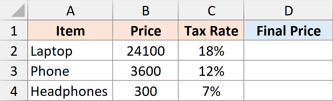
I want to calculate the final price, which is going to be the given price with the tax added to it.

Now I can do this with a simple multiplication formula in Excel, but let me show you how to do this using the LET function.

Enter the below let formula in cell D2.

=LET(
price,B2:B4,
taxrate,C2:C4,
price*(1+taxrate))

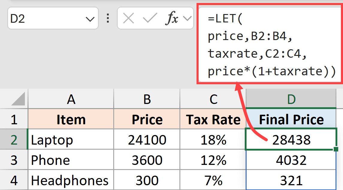
Here is what is happening:

• I have used a variable called price and then assigned the values in B2:B4 to this variable.
• Then I’ve used a variable called taxrate and assigned the values in C2:C4 to this variable.
• And since the last argument of the LET function should always be a calculation, I have used the calculation price*(1+taxrate))

The LET function returns the value given by the calculation, where the calculation is in turn using the variables that I have defined in the previous arguments.

Now I think I know what you’re thinking, and let me address it.

For this specific example, you would be better off simply using a formula where you manually refer to the cell that has the price and add tax to it.

Something like:

=B2*(1+C2)

And you’re absolutely right in thinking so.

In this specific example, we do not really need to use the LET function. But I wanted to show you how you can use LET to assign variables to values and then use that in a calculation.

As we move to more complex examples, you would notice that it becomes a lot easier to refer to values when a name has been assigned to it in a complex calculation rather than using cell references.

Also read: 100+ Excel Functions Explained

Example 2 – Restructure Full Name with Text Functions

Now, let’s look at an example where let actually makes the formula a little easier to manage.

Below, I have a dataset where I have the full name in column A (in the fromat FirstName LastName), and I want to modify these names so that they appear in the LastName-FirstName format.

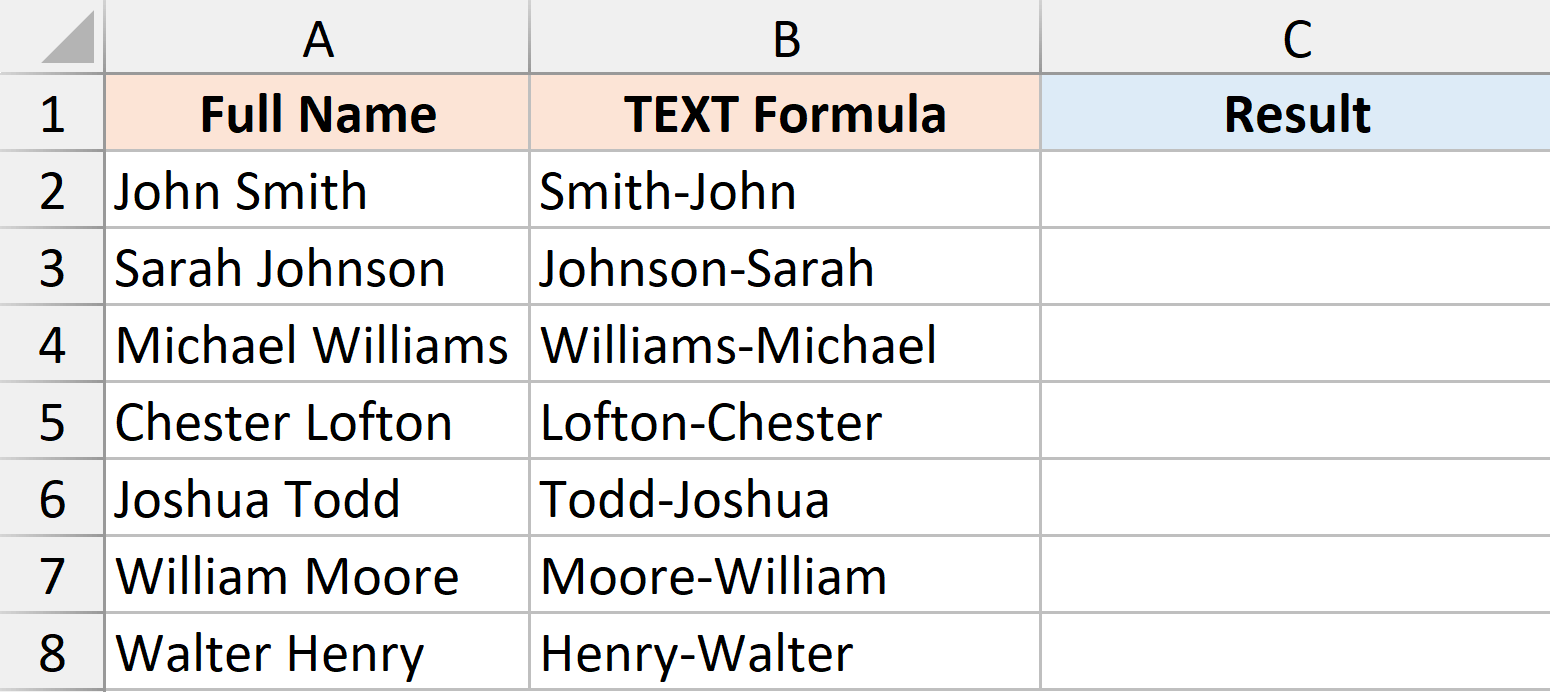
So for John Smith, I want the result to be Smith-John.

Now, if I have to do this using the regular text functions, I can use the below formula.

=RIGHT(A2, LEN(A2) - FIND(" ", A2))&"-"&LEFT(A2, FIND(" ", A2) - 1)

But let me show you how to do this using the LET function.

Below is the LET formula that would give us the result.

=LET(
name,A2:A8,
fn,LEFT(name, FIND(" ", name) - 1),
ln,RIGHT(name, LEN(name) - FIND(" ", name)),
ln&"-"&fn)

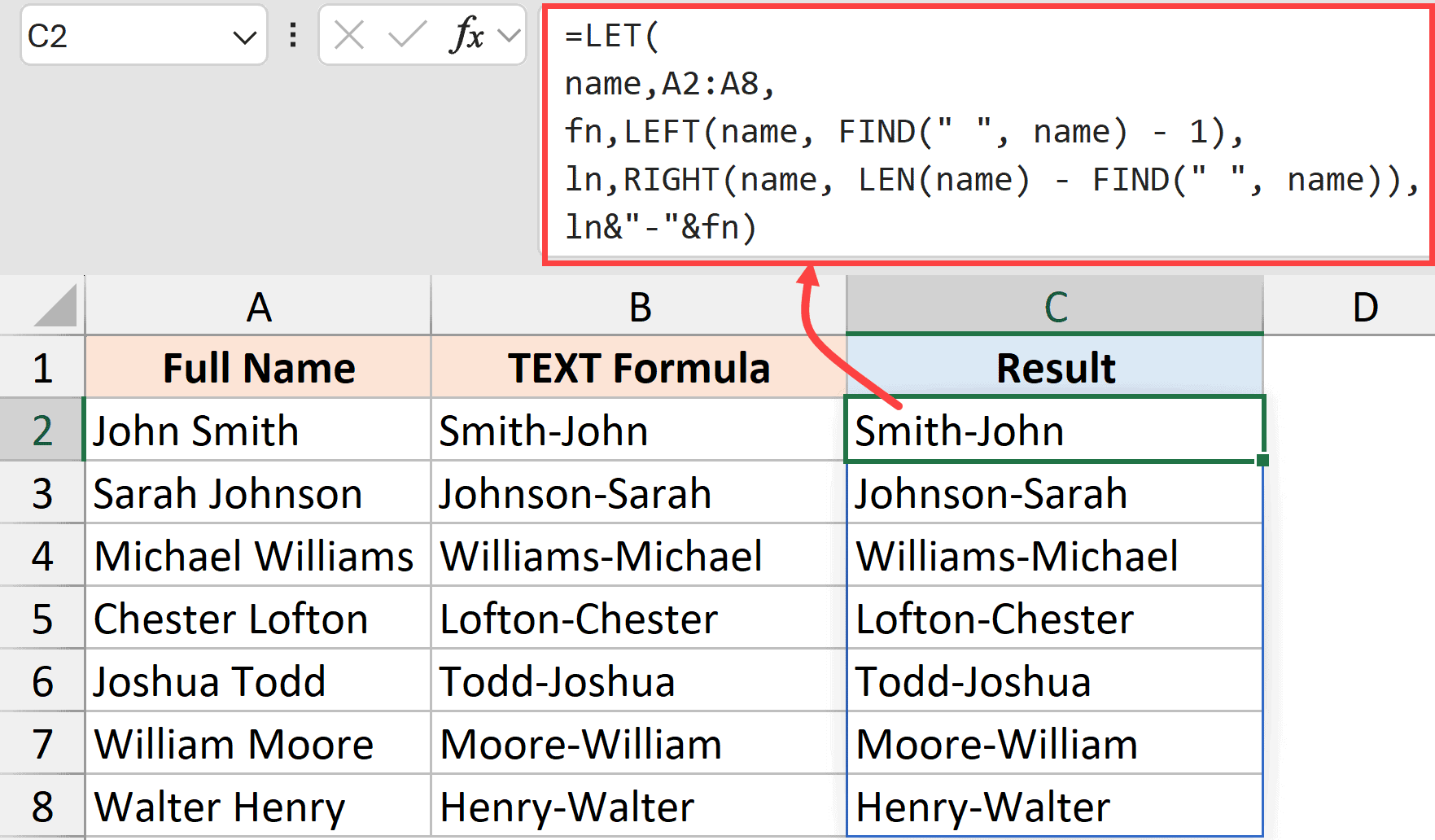
Here is what is happening in the above formula.

• name is a variable that stores the range of cells that contain the names.
• fn variable is used to store the value of LEFT(name, FIND(” “, name) – 1). This will give me the first name from each cell.
• ln variable is used to store the value of RIGHT(name, LEN(name) – FIND(” “, name)). This will give me the last name from each cell.
• ln&”-“&fn – this is the calculation that gives me the desired result.

The benefit of using this formula is that since I have the first name and the last name stored in two separate variables, if I need to change the format of the name I want, I can simply change the last argument.

For example, if I want to get the first name followed by a dash and then the last name, I can simply change the last argument to fn&”-“&ln

So while you may not see it as a shorter formula, this certainly becomes a more manageable formula.

Now, if you are still not convinced, let me show you another example where let leads to a significant improvement in the readability of the formula.

Also read: Separate First and Last Name in Excel

Click here to download the example file

Example 3 – Calculating Student’s Grades

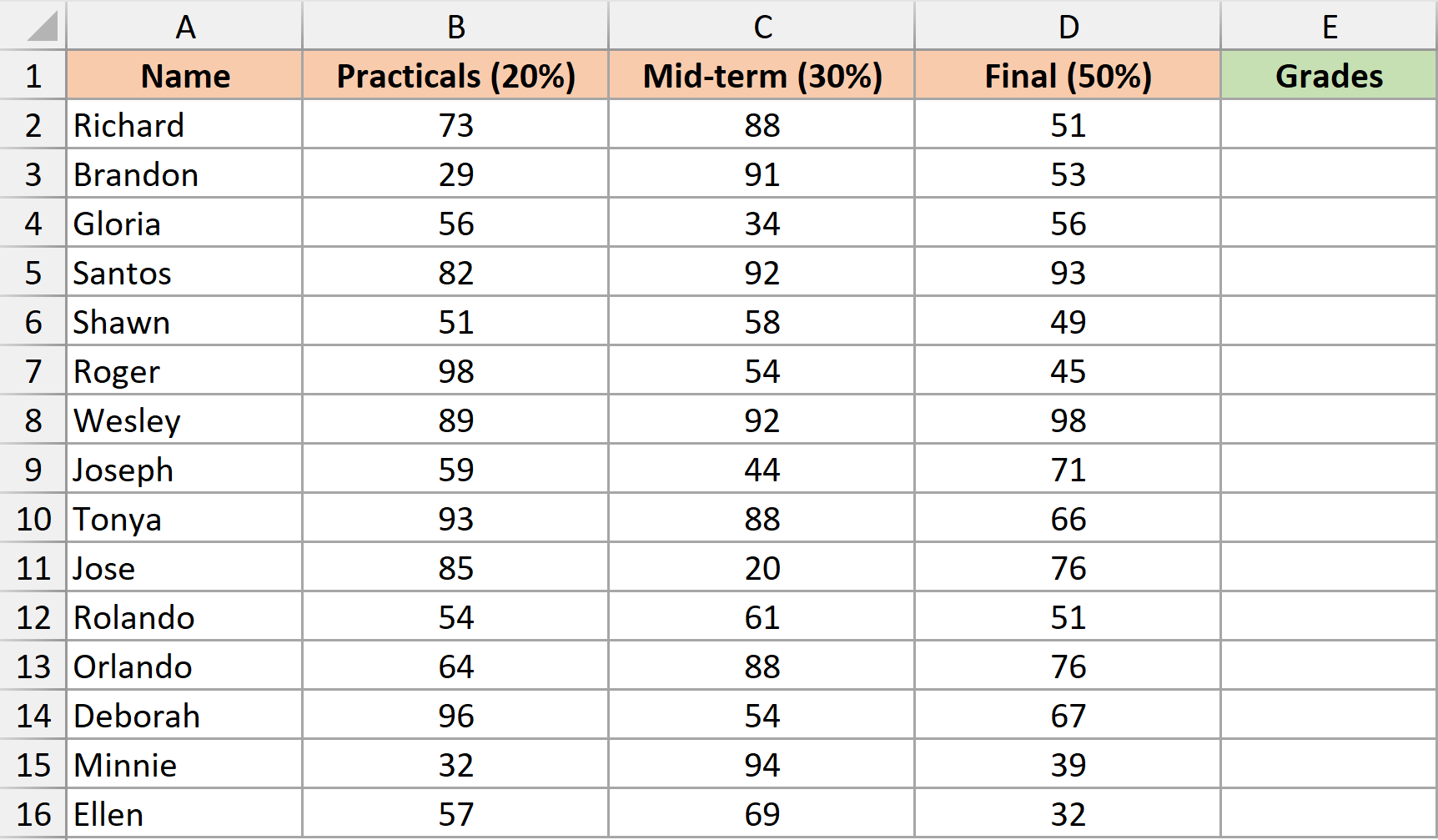
Below, I have a dataset where:

• Student names are in column A
• Practicals score in column B (weightage – 20%)
• Mid-term score in column C (weightage – 30%)
• Final exam score in column D (weightage – 50%)

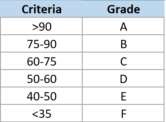
Now I have to calculate the grade for each student based on the following criteria:

This is a classic nested if situation, and if I am using a regular IF function to solve this, here is the formula I will have to use:

=IF((B2*0.2+C2*0.3+D2*0.5)>90,"A",IF((B2*0.2+C2*0.3+D2*0.5)>75,"B",IF((B2*0.2+C2*0.3+D2*0.5)>60,"C",IF((B2*0.2+C2*0.3+D2*0.5)>50,"D",IF((B2*0.2+C2*0.3+D2*0.5)>40,"E","F")))))

That looks a bit scary. Is it not?

Now here is the same thing done using a LET formula.

=LET(wts,B2:B16*0.2+C2:C16*0.3+D2:D16*0.5,
IF(wts>90,"A",
IF(wts>75,"B",
IF(wts>60,"C",
IF(wts>50,"D",
IF(wts>40,"E","F"
))))))

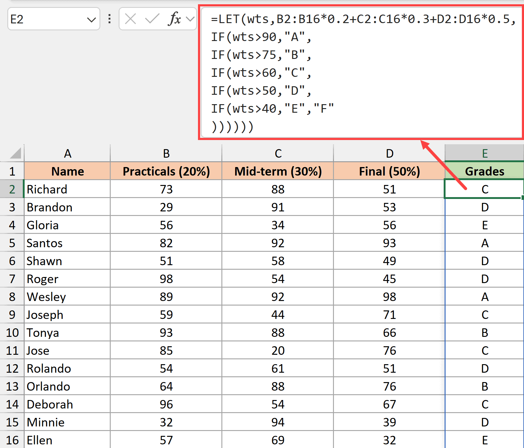
The LET function in this example is better than the nested IF formula because it makes your formula more manageable.

For example, if I adjust the weightage where practicals and mid-terms both get 25% weightage, I just need to make the change once in the let formula. But in the nested if function, you’ll have to make the change in multiple places.

I can’t tell you how many times I’ve messed up my nested formulas because I forgot to make the change in one of the places. LET formula certainly solves that problem.

Click here to download the example file

Example 4 – LET Formula to Get Result in Multiple Columns

Now let me show you how one single LET formula that spills over and give the results in multiple columns.

Below, I have a dataset where I have names in column A, units sold by them in column B, the price per unit in column C, and their commission % in column D.

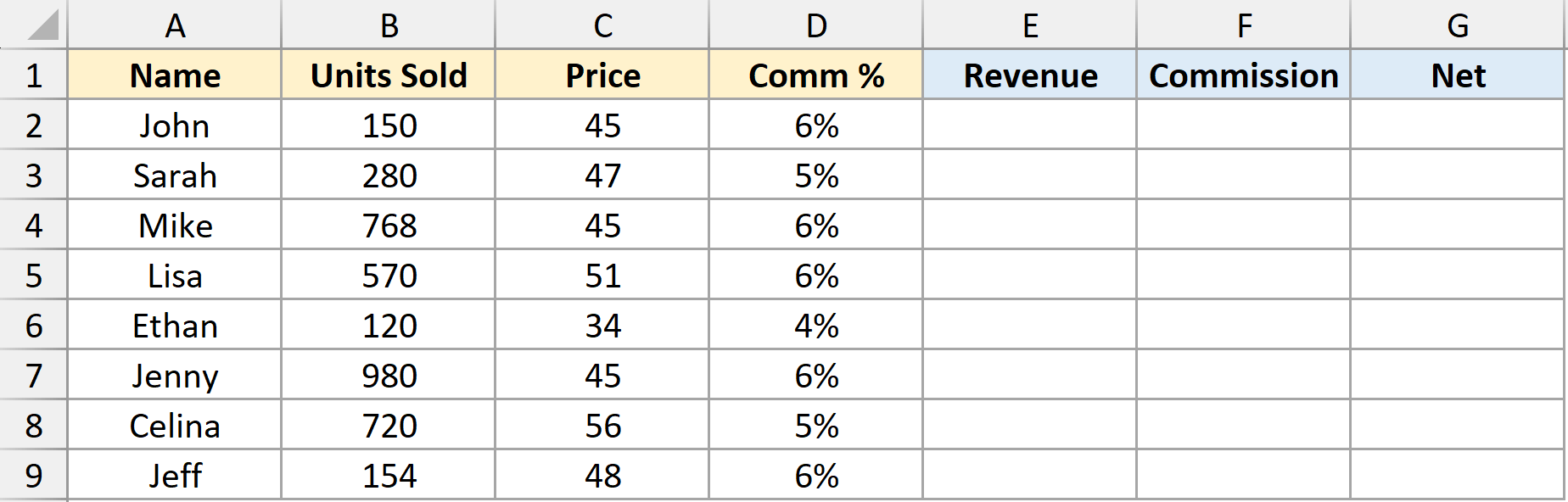
Now for each row, I want three different values:

• Revenue by each person
• Commission earned
• Net Revenue after the Commissions have been paid

Normally, this would be done by using three different formulas for the three different columns.

But here is a LET formula that will spill over and give you the results in all three columns.

=LET(
price, C2:C9,
comper, D2:D9,
revenue, B2:B9 * price,
commission, revenue * comper,
net_revenue, revenue - commission,
CHOOSE(
{1,2,3},
revenue,
commission,
net_revenue
))

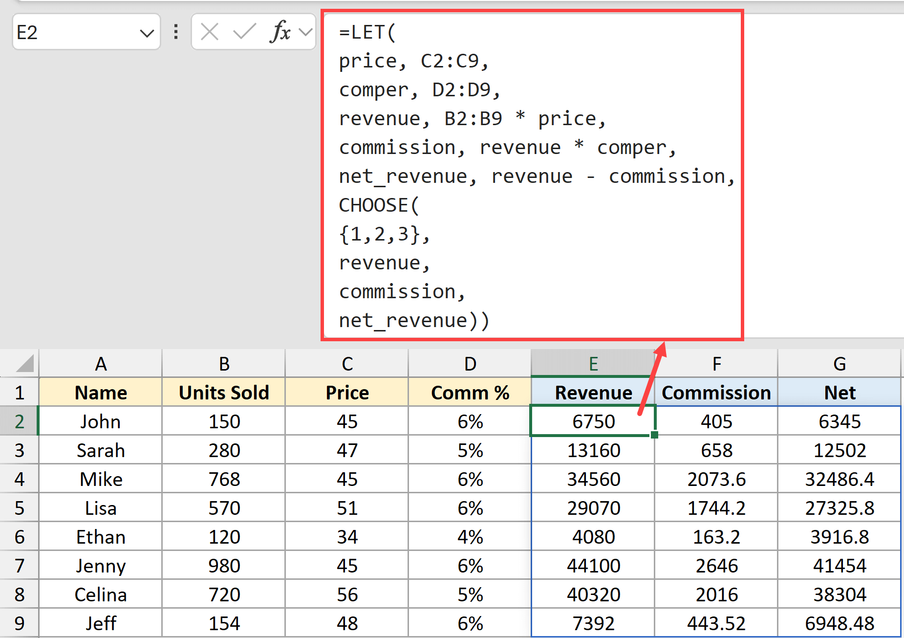
In the above formula:

• C2:C9 is assigned to a name price
• D2:D9 is assigned to a name comper
• Revenue is calculated by using B2:B9 * price
• Commission is calculated using revenue * comper (and the result is assigned to a name called commission)
• Net revenue is calculated using revenue – commission and is assigned to a name net_revenue

Once all the name assignments are done, I have used the CHOOSE function to return the result in three different columns:

1. The first column gets the revenue values
2. The second column gets the commission values
3. The third column gets the net_revenue values

The good thing about using this formula is that you don’t need to make the changes in three different places in case anything changes. You can make all the changes in one single formula, and the result in all the three columns will automatically update.

Using these kinds of LET functions can help minimize errors, as you only need to check everything in one single formula insetad of checking formula in each column.

Now that you understand the concept of using LET function that spills over multiple columns, let’s see a couple of practical examples.

Click here to download the example file

Example 5 – Creating Full Ammortization Schedule with One Formula

In this example, I will show you how to create a full amortization schedule with a single LET formula.

Here are the data points I’ll be using in the formula.

• Principal amount = 100000
• Duration in months = 60
• Annual interest rate = 4%

Here is the formula that will give you the titles as well as the entire amortization schedule in the result:

=LET(
loanamount, 100000,
timeperiod, 60,
monthlyInterest, 4%/12,
InterestPayment, PMT(monthlyInterest,timeperiod,loanamount,0),
PrincipalBalance, loanamount-ABS(CUMPRINC(monthlyInterest, timeperiod, loanamount, 1, SEQUENCE(timeperiod), 0)),
headers, {"Time","Balance","Payment"},
result, CHOOSE({1,2,3},
SEQUENCE(timeperiod),
InterestPayment,
PrincipalBalance),
VSTACK(headers,result))

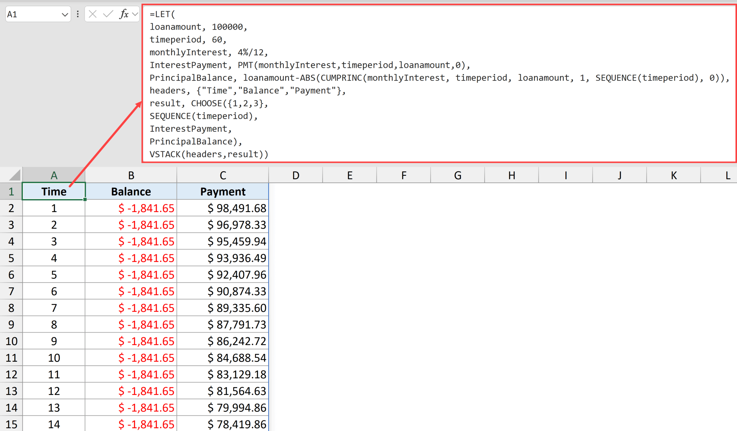
Now, this might look a bit daunting at first, but if you go through this formula step-by-step, you will realize that all we have done is bring all the steps that are needed to calculate the amortization schedule within one single formula.

Let me explain how it works line by line:

• loanamount, 100000, – The loan amount value of $100,000 is assigned to a variable called loanamount.
• timeperiod, 60, – The number 60 is assigned to a variable called timeperiod. This represents the total number of monthly payments (5 years × 12 months = 60 payments).
• monthlyInterest, 4%/12, – The annual interest rate of 4% is divided by 12 to get the monthly interest rate, and this is assigned to a variable called monthlyInterest. Since loans compound monthly, we need the monthly rate for calculations.
• InterestPayment, PMT(monthlyInterest,timeperiod,loanamount,0), – The PMT function calculates the fixed monthly payment amount for a loan. It takes the monthly interest rate, number of payments, and loan amount as inputs. The result (your monthly payment) is assigned to the variable InterestPayment.
• PrincipalBalance, loanamount-ABS(CUMPRINC(monthlyInterest, timeperiod, loanamount, 1, SEQUENCE(timeperiod), 0)), – This calculates the remaining loan balance after each payment. CUMPRINC calculates the cumulative principal paid up to each month, ABS makes it positive (since CUMPRINC returns negative values), and subtracting this from the original loan amount gives us the remaining balance. SEQUENCE(timeperiod) creates a list of numbers 1 through 60 for each month.
• headers, {“Time”,”Balance”,”Payment”}, – Creates the column headers for our amortization table and assigns them to the variable “headers”.
• result, CHOOSE({1,2,3}, SEQUENCE(timeperiod), InterestPayment, PrincipalBalance) – The CHOOSE function creates three columns of data:
  • Column 1: SEQUENCE(timeperiod) creates month numbers 1, 2, 3… up to 60
  • Column 2: InterestPayment repeats the same monthly payment for all rows
  • Column 3: PrincipalBalance shows the remaining balance after each payment
• VSTACK(headers,result)) – since this is the last argument in the formula, this is the value that is returned as the result of the formula. VSTACK combines the headers row with the data rows vertically, creating a complete table with headers at the top and all the amortization data below.

The final result is a complete amortization schedule showing the payment number, remaining balance, and monthly payment amount for each month of the loan.

I know this looks like a handful, but using the LET formula offers several advantages over using individual formulas:

• One Single formula – Everything is within one formula compared with multiple different formulas in different cells
• Easy updates – If you want to modify anything, you just need to make the change in this one formula. For example, if the loan amount changes or you want the details for more or less number of periods, you need to make the changes in one place only.
• Reduced errors – More formulas mean more chances of errors. With this formula, you will be dealing with one formula only (so if something is wrong, you know where to look).
• Easier to Copy to Other Sheets/Workbooks – Copy to other worksheets without worrying about missing dependencies
• Better documentation – It is easier to document one single formula rather than documenting multiple formulas that are scattered across the worksheet.

In this article, I’ve tried to give you an overview of the LET function by explaining some simple examples and I’ve also shown you how it could be a really powerful tool when you’re working with long, complex formulas.

While it took me some time to warm up to the LET function, now always look for opportunities to simplify my complex formulas with this function.

I hope you found this article helpful. If you have any questions or suggestions for me, please let me know in the comments section.

Other Excel articles you may also like:

• Excel LAMBDA Function
• 20 Advanced Excel Functions and Formulas (for Excel Pros)
• VLOOKUP vs XLOOKUP Function – What’s the Difference?
• Excel XLOOKUP Function (10 Examples)