Sort Pivot Table in Excel

Pivot Tables come with a lot of in-built sorting options that allow you to structure your data the way you want.

While you can use the regular sorting options (sorting A-Z / Z-A or Smallest to Largest or Largest to Smallest), there are also options to sort based on a custom list and even specify the sorting order manually.

In this article, I will cover everything you need to know about sorting Pivot Tables in Excel.

Click here to download the example file

Sort Rows or Columns Area

When you create a Pivot Table, the rows and the columns area are automatically sorted in an ascending order.

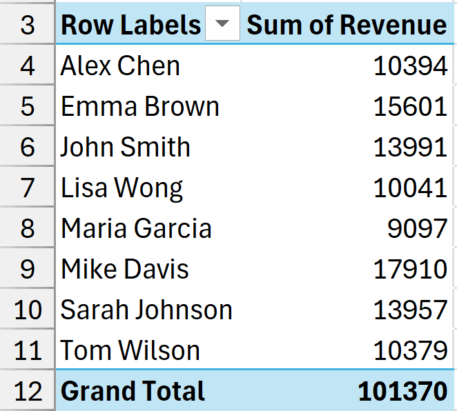
For example, in the below Pivot Table, you can see that the Salesperson names in the row area and the Category names in the column area are sorted alphabetically in an ascending order from A to Z.

If you want to change the sort order, here’s how to do it.

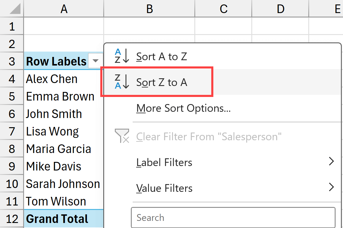
1. Click on the drop-down icon in the Salesperson’s cell.
2. Select from the options to Sort A to Z or Sort Z to A. In this example, let’s choose the Sort Z to A option.

Alternatively, you can also select any cell in the column, then go to the Data tab, and click on the sort icons.

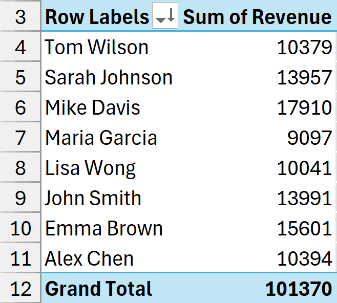
This will give you the dataset as shown below.

Now here is an interesting thing about sorting in pivot tables.

When you apply a sort order to a column, the PivotTable is going to remember it and even if you change the structure of your PivotTable, that sort order would still be maintained.

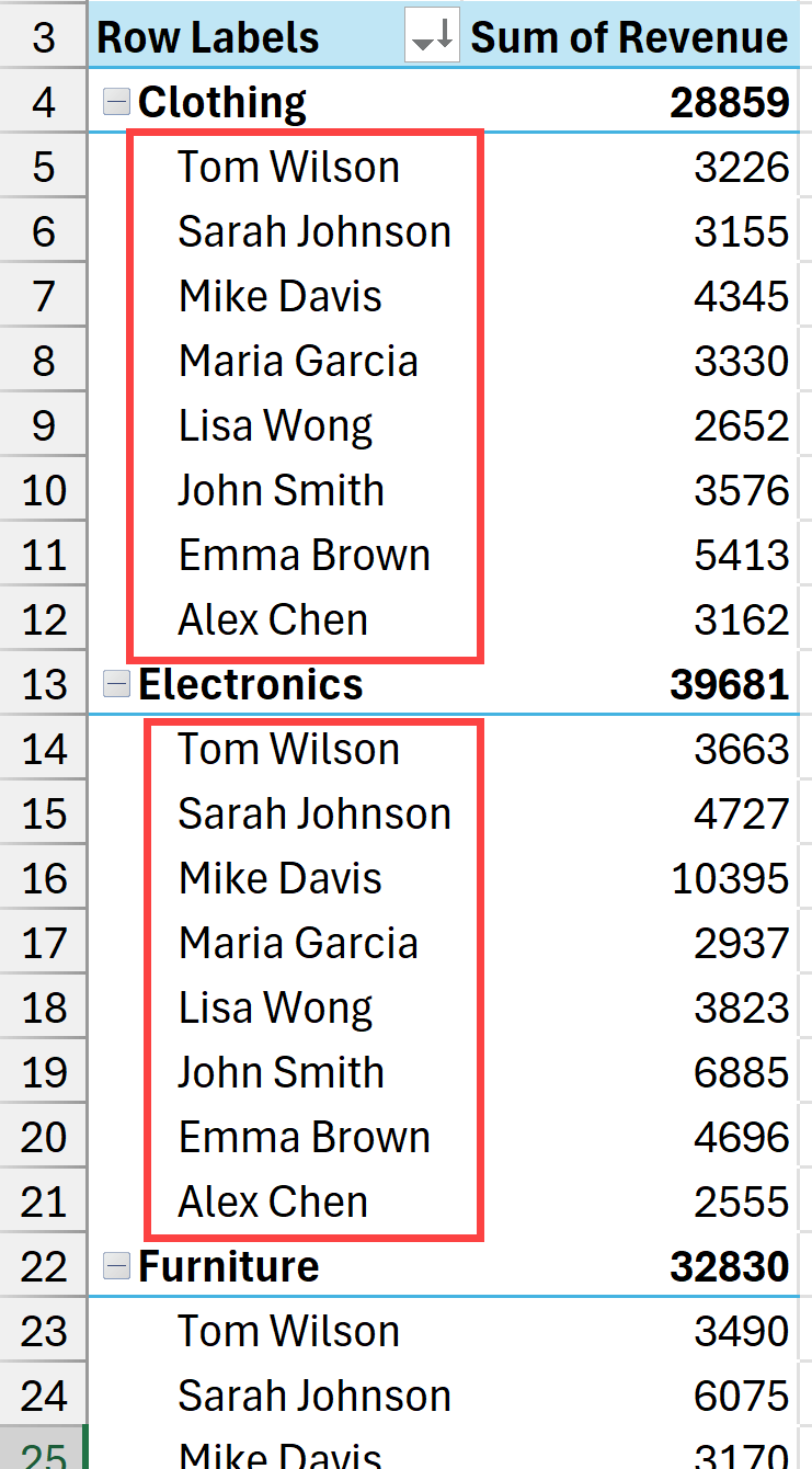
For example, if I add the Category option to the rows area as well, you will notice that within each Category, the names data is still sorted in the descending order.

Even if you remove the salesperson’s names data from the Pivot Table and then add it back, it would still be sorted in the descending order.

Similarly, if you want to sort the data in the columns area, you can do the same thing by:

1. Clicking on the drop-down in the column label cell and then choosing the sort order, or
2. Selecting any cell in the columns area and then using the sort options in the Data tab

Important Note: When you create a Pivot Table, the sorting preference is given to custom lists that are already saved in your Excel application. This is why when you create a pivot table that has month names, those would be listed chronologically (January, February, March) and not alphabetically. If there are no custom lists relevant for your dataset, then your data would be sorted in an alphabetically in an ascending order.

Click here to download the example file

Sort the Values Area

In most cases, you would want to apply sorting to the values area in your pivot table.

For example, in the below Pivot Table, I want to sort the Clothing column in a descending order (from largest to smallest).

Here are the steps to do this:

1. Select any cell in the Clothing column (or any column based on which you want to do the sorting)
2. Click the Data tab in the ribbon.
3. Click on the Sort Largest to Smallest icon (the Z to A icon)

Alternatively, you can also right-click on any cell in the Clothing column and go to the Sort option and click on the Sort Largest to Smallest option.

This will sort the Clothing column in descending order.

Unlike the row and column area level sorting (where Pivot Table remembers the sorting that you applied) in case of the values area, it won’t.

For eg., if I remove the revenues value and add it back again, it would forget that I sorted the clothing column in a descending order. It would revert to showing the sales rep names in the alphabetical order or whatever sorting has been applied on that column.

Sort Left to Right in Values Area

You can also sort the data set in a Pivot Table from left to right.

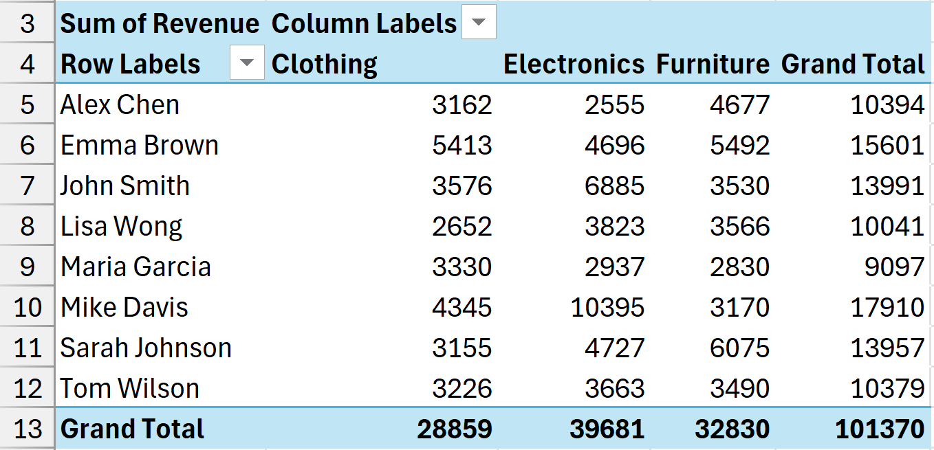
Below I have a pivot table where I have:

• Salespeople’s names in the rows area
• Categories in the columns area
• Values showing the sum of sales

Now, in this Pivot Table, I want to sort the data for Emma Brown from largest to smallest.

Here are the steps to do this:

1. Select any cell in the row that shows the values for Emma Brown.
2. Click the Data tab in the ribbon.
3. Click on the Sort icon.

4. In the Sort by Value dialog box that opens, select the following:
   • Sort options – Largest to Smallest
   • Sort direction – Left to Right

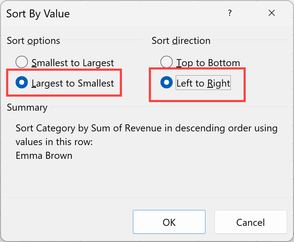
5. Click OK

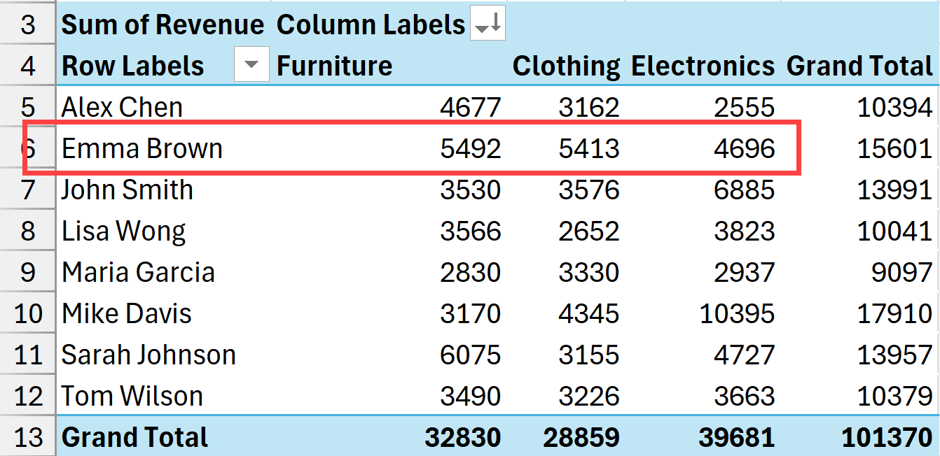
This will sort the Pivot Table based on the values in the row for Emma Brown.

Sorting the Outer Row Field in Pivot Table

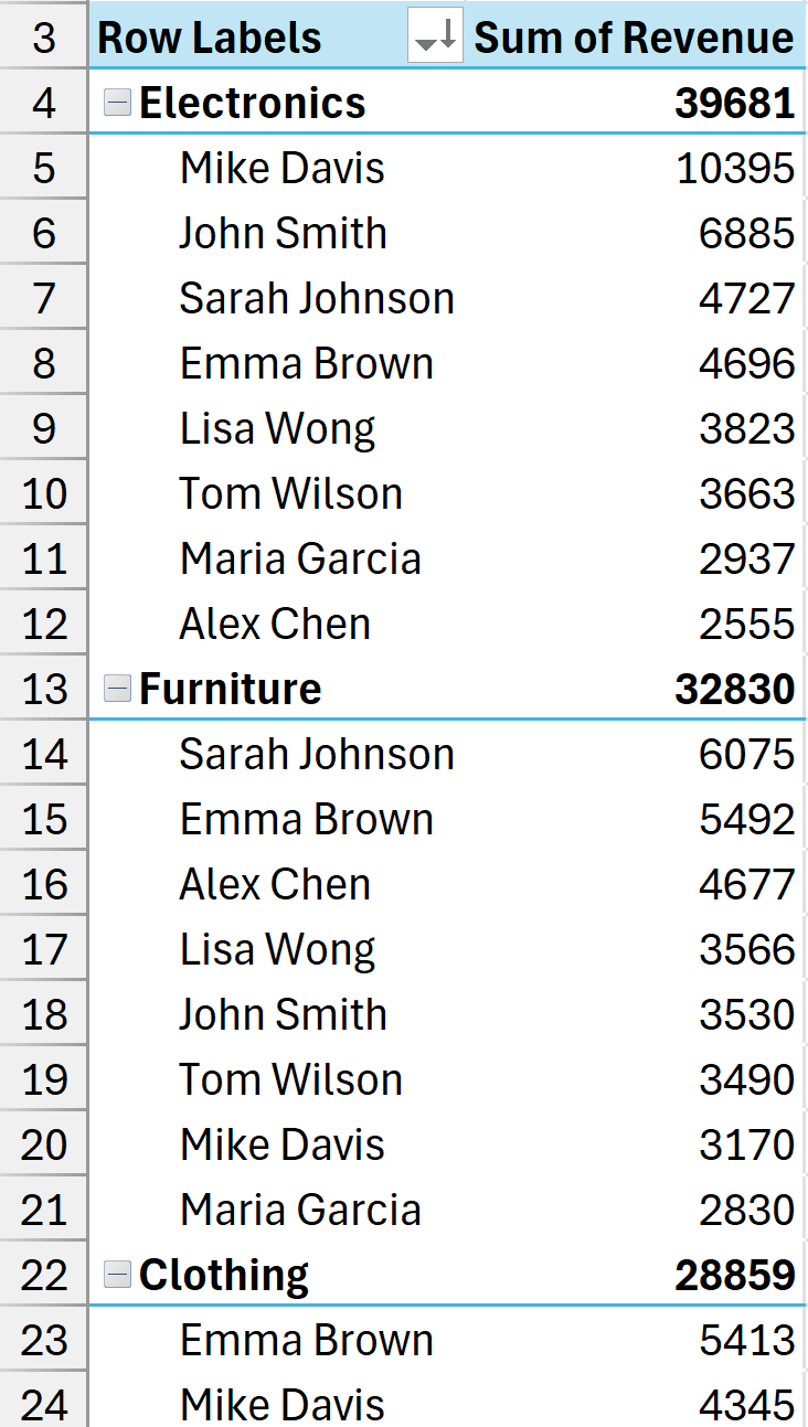
Below I have a pivot table where I have already sorted the data based on sales value in a descending order. So the person with highest sales shows up at the top and the one with lowest shows up at the bottom.

Now, if I add the Category as the outer field in this Pivot Table, you will get something as shown below:

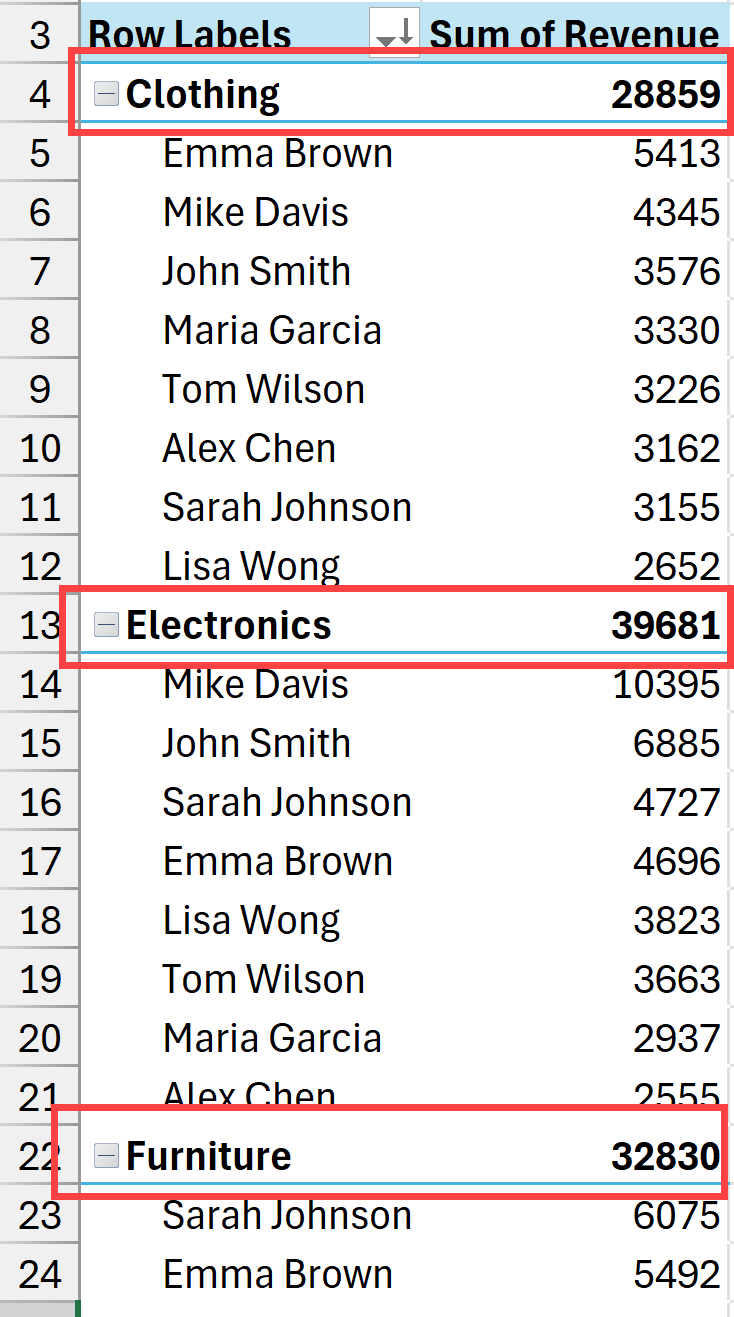
Now you can see that while the salesperson’s names are sorted in a descending order based on their sales values, the outer category (which has Clothing, Electronics, and Furniture) is not sorted based on the total sales values (it’s sorted alphabetically).

It would be more useful if the category is also sorted in the descending order, where the one with the largest sales is shown at the top.

And this can be fixed easily.

Pivot Table considers the outer field and the inner field as separte datasets, and you can apply the same or different sorting criteria to each of these fields.

So, if in this example I want the outer field to be sorted in a descending order as well, I would select any cell in the values area corresponding to the outer field and apply the sorting (using the sort icons in the Data tab in the ribbon).

For example, if I choose cell B4 and apply the descending sort order. I’ll get something as shown here.

Sorting the outer field will not disturb the sorting already applied on the inner field.

Click here to download the example file

Manual Sorting in Pivot Tables

Pivot Tables also have an interesting Manual sorting option where you can set the sorting criteria by manually rearrangging the rows and columns around.

Below, I have a Pivot Table where I have the salesperson’s name in the rows area and the product category in the columns area.

By default, my Pivot Table is sorted in the alphabetical order (for both Salesperson’s name and the Category names).

Now let’s say that I want to focus on the Furniture category and would like it to show up at the first column.

Here are the steps to manually do this:

1. Select the Furniture column label, which is the cell that contains the text Furniture.
2. Place the cursor around the edge of the selection. You’ll notice that your cursor changes to a four-arrow pointed icon.

3. Press the left mouse key and then drag the cell to the position where you want it. You will see a thick green line as you are moving the cursor. Bring the line where you want the column and then leave the mouse key. In this case, I will drag it right next to the Salesperson column

By doing this, I have sorted my Pivot Table manually, where Furniture becomes the first column, and all the remaining columns shift to the right.

Another way to do manual sorting is to simply change the column label. For example, if I want the furniture column to appear instead of the clothing column, I can just change the word ‘Clothing’ to ‘Furniture’ and as soon as I hit Enter, Pivot Table would understand that I want to do the manual sorting, so it will bring the Furniture column in place of the Clothing column and shift the Clothing column to the right.

Caution when using Manual Sorting:

• There is no visual indication showing that manual sorting has been done (except that my column label data is not sorted in the alphabetical order).
• When you sort a column in an ascending or descending order, and then you use manual sorting, it is going to redo the sorting based on what column now appears in its position. For example, if my data was sorted based on the Clothing column in a descending order, and then I apply manual sorting, it will then sort based on whatever column takes the position of the Clothing column. This is non-intuitive and can be confusing.

Click here to download the example file

Sort Using Custom List

You can also create your own custom lists that can be used for sorting the data in the rows and columns area in your Pivot Tables.

Custom lists get priority when it comes to sorting pivot tables. So if you already have a custom list, Pivot Table will first use that to apply the sorting criteria, and if there is no relevant custom list, it will sort alphabetically.

Excel already has four built-in custom lists.

• Sun, Mon, Tue,….
• Sunday, Monday, Tuesday….
• Jan, Feb, Mar,….
• January, February, March,….

This is why when you add dates to the rows or columns area and show the data based on days or months, it is going to use these built-in custom lists to arrange the data.

Below is an example where I have added Months (Date) in the Rows area and Revenue in the columns area.

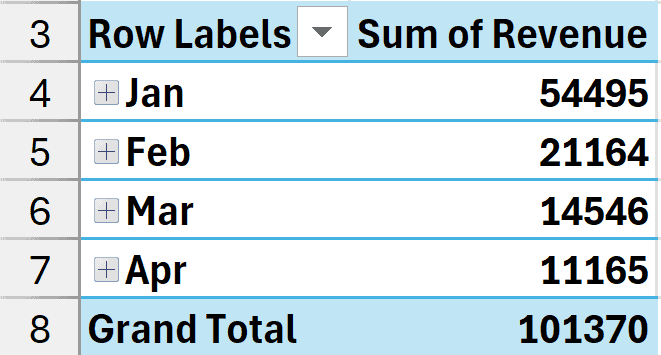
You can see that it automatically puts January at the top, followed by February, March, and so on (which makes sense).

You can also create your own custom list that would be used by default when you create any new Pivot Table.

For example, let’s say I have the same data and I always want to show my data in the following order: Furniture –> Clothing –> Electronics

Here are the steps to create your own custom list:

1. Click the File tab.

2. In the backstage area that opens, click on Options.
3. In the Excel Options dialog box, click on the Advanced option in the left pane.

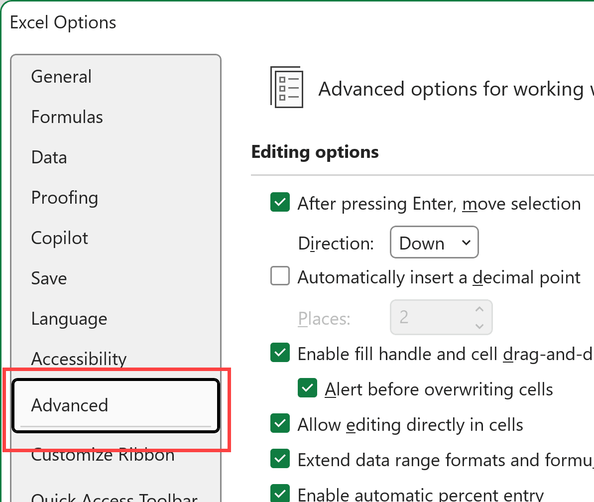
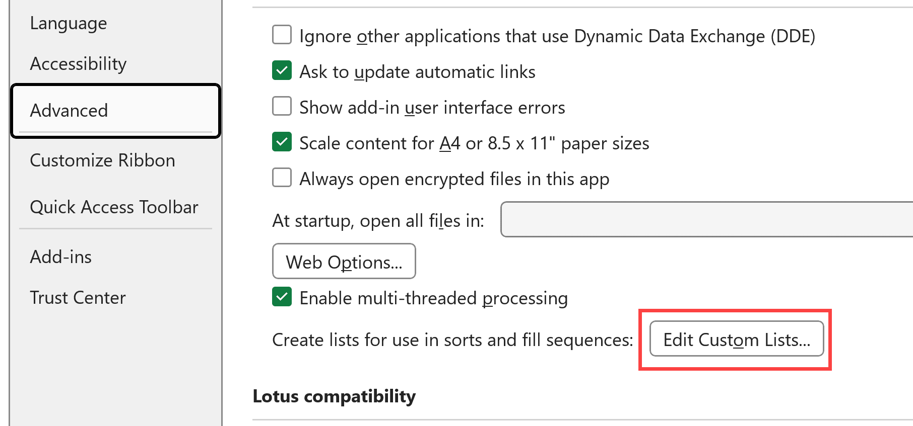
4. Scroll down and at the bottom, you’ll find a button called Edit custom lists. Click on it.

5. In the Custom List dialog box, enter the custom list you want in the List Entries box. Put each item on a separate line.

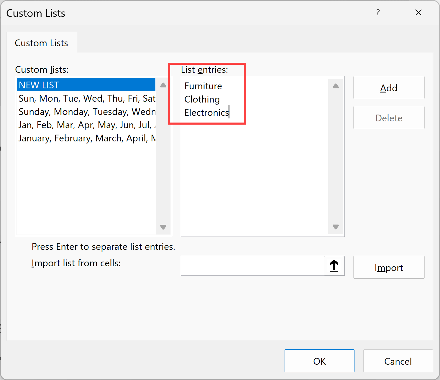
6. Click on Add

The above steps would create a custom list that would now be used when you create any new pivot table.

When I manually enter the items in the custom list, you can also have these items in a range in Excel and then import it into the custom list dialog box.

So now, if I create my pivot table again from scratch from the source data and then put the category field in the columns area, it would automatically sort it using the custom list I created.

This article covered everything you need to know about sorting in Pivot Tables and some sorting tricks that you can use to help you get the data in the structure that you want.

I hope you found this article helpful. In case you have any questions or suggestions, please let me know in the comments section.

Other Excel and Pivot Table articles you may also like:

• Group Numbers in Pivot Table in Excel
• Change Pivot Table to Tabular Form
• Pivot Table Keyboard Shortcuts
• Connect a Single Slicer to Multiple Pivot Tables
• Using Slicers in Excel Pivot Table