

If you want to look up a value using two or more conditions at once, a regular lookup won’t get you there. It can only match on a single column, so the moment two rows share the same name (or the same month), it just grabs the first one it finds.
The fix is to combine INDEX and MATCH so they check both conditions together. It’s easier than it looks, and in this article I’ll show you how to do a multiple criteria lookup with INDEX MATCH, plus a simpler helper column version.
INDEX MATCH with Multiple Criteria Using an Array Formula
This is the classic approach, and it’s the one I reach for most.
It checks both conditions in a single formula and returns the value where both are true, without you having to add any extra columns.
Let me show you how it works.
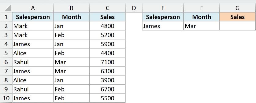
Below I have a small sales dataset. Column A has the salesperson, column B has the month, and column C has the sales amount. The same salesperson shows up in multiple months, so the name alone isn’t enough to find one specific number.
I want to pull the sales for a given salesperson in a given month. I’ve typed the two things I’m looking for into cells E2 (the salesperson) and F2 (the month).
Here is the formula:
=INDEX(C2:C10, MATCH(1, (A2:A10=E2)*(B2:B10=F2), 0))
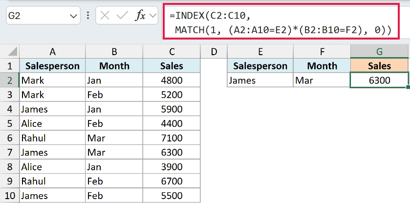
With “James” in E2 and “Mar” in F2, this returns 6300, which is exactly the number sitting where those two conditions meet.
How does this formula work?
The trick is in the middle part, where the two conditions get multiplied together.
(A2:A10=E2) checks each salesperson against E2 and gives back a list of TRUE and FALSE values, TRUE wherever the name is James.
(B2:B10=F2) does the same thing for the month, giving TRUE wherever it says Mar.
When you multiply those two lists together, Excel turns TRUE into 1 and FALSE into 0. You only get a 1 in the rows where BOTH conditions are true, so the multiplication is doing the job of an AND.
MATCH(1, ..., 0) then finds the position of that first 1 in the list. The 0 tells MATCH to look for an exact match.
Finally, INDEX takes that position and returns the matching value from the sales column. In this example the match is in the 6th position, so INDEX pulls the 6th value from C2:C10.
There’s one important thing to know about entering this formula, depending on your Excel version.
In Excel 365 and Excel 2021, you just type it and press Enter. Dynamic arrays handle the behind-the-scenes list on their own.
In Excel 2019 and earlier, this is an array formula, so you have to press Ctrl + Shift + Enter instead of Enter. Excel then wraps it in curly braces. Skip that step in the older versions and you’ll get an error or the wrong result.
Pro Tip: If you’re on Excel 365 or 2021, XLOOKUP can do the same two-criteria lookup with less typing: =XLOOKUP(1, (A2:A10=E2)*(B2:B10=F2), C2:C10). It uses the exact same TRUE/FALSE multiplication trick, and you just press Enter.
INDEX MATCH with a Helper Column
If array formulas make you nervous, or you’re on an older version and don’t want to deal with Ctrl + Shift + Enter, a helper column is a clean alternative. You mash the two criteria into a single column and then do a normal, everyday lookup against it.
Here’s the same dataset. Salesperson in column A, month in column B, sales in column C, and the two things I’m looking for in F2 and G2.
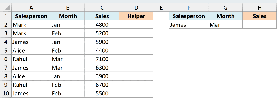
First, add a helper column (I’ll use column D) that joins the salesperson and the month together. In cell D2, enter:
=A2:A10&"|"&B2:B10
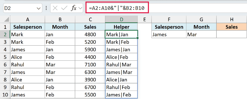
In Excel 365 and 2021 this spills down the whole column automatically, so you get Mark|Jan, Mark|Feb, and so on down the list. In older versions, put =A2&"|"&B2 in D2 and copy it down.
The "|" in the middle is a separator. It keeps the two pieces apart so two different combinations can’t accidentally collapse into the same text.
Now you can do a plain INDEX MATCH against that helper column:
=INDEX(C2:C10, MATCH(F2&"|"&G2, D2:D10, 0))
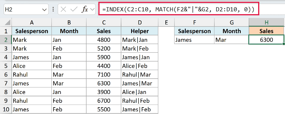
F2&"|"&G2 builds the same combined text you’re looking for, James|Mar. MATCH finds where that appears in column D, and INDEX returns the sales value from the matching row, 6300.
This version isn’t an array formula, so it works the same way in every version of Excel with just the Enter key. The only cost is that extra column, which you can tuck away or hide if you don’t want to see it.
Things to Keep in Mind
- Add more criteria by multiplying in another condition. Say you also had Region in column C, with the sales amounts moved over to column D, and the region you want in G2. You would use
=INDEX(D2:D10, MATCH(1, (A2:A10=E2)*(B2:B10=F2)*(C2:C10=G2), 0)). Each condition you multiply in has to be true for that row to score a 1. - Always use 0 (or FALSE) in MATCH. The 0 forces an exact match. Leave it out and MATCH switches to approximate match, which needs sorted data and will give you the wrong row here.
- The separator in the helper column matters. Joining “12” and “34” gives “1234”, and so does joining “123” and “4”. A separator like
|between them prevents those false matches. - This handles left lookups, which VLOOKUP can’t. Because INDEX pulls from any column you point it at, your answer column can sit to the left of your criteria. If you’d rather stick with VLOOKUP, here’s how to do a VLOOKUP with multiple criteria.
If you want a deeper walkthrough of how these two functions work together on a single criterion, I’ve covered the full INDEX MATCH combo separately. And if you’re still deciding between approaches, the plain VLOOKUP function guide is a good starting point.
I hope you found this article helpful.
Other Excel Articles You May Also Like:
