

If you want to check whether two or more conditions are true at the same time, a plain IF function won’t get you there.
For example, you may want to pass a student only if they scored at least 50 and also have 75% attendance.
That’s because IF only tests one condition at a time.
Good news is this is easy to solve. You just nest the AND function inside IF, and in this article I’ll show you how to use IF with AND to test several conditions at once.
Follow along with the example file
IF with AND Excel.xlsx
How the AND Function Works
Before we combine it with IF, here’s a quick look at what AND does on its own.
AND checks whether every condition you give it is true. If all of them are true, it returns TRUE. If even one is false, it returns FALSE.
You can give it up to 255 conditions, and they all have to be true for the result to be TRUE.
If you want the full rundown with more examples, check out my guide on the AND function.
IF with AND: Check Two Conditions
The AND function on its own only gives you TRUE or FALSE. Most of the time you want something more useful, like a label that says who passed.
That’s where IF comes in. You put the AND test inside the IF function, and IF shows one result when the test is true and another when it isn’t.
Below I have a list of students, with their exam score in column B, their attendance in column C, and the number of assignments they submitted (out of 10) in column D.
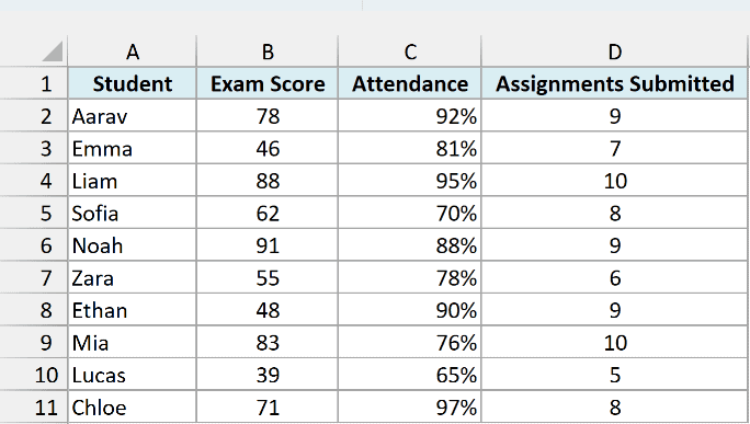
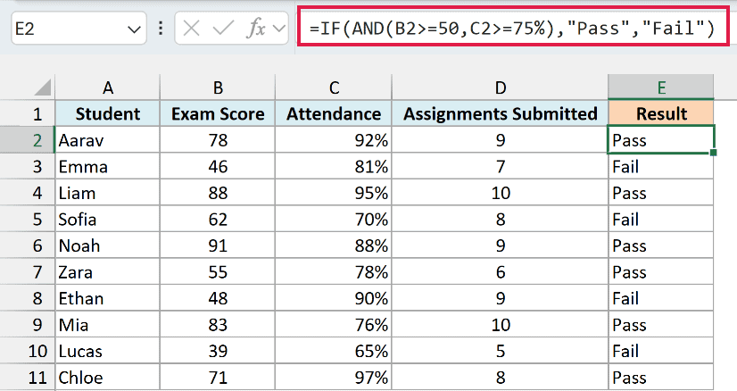
I want to mark a student as “Pass” only when their exam score is at least 50 and their attendance is at least 75%. Everyone else gets “Fail”.
Here is the formula:
=IF(AND(B2>=50,C2>=75%),"Pass","Fail")
How does this formula work?
AND(B2>=50,C2>=75%) is the logical test. It’s TRUE only when the score is 50 or more and the attendance is 75% or more.
When the test is TRUE, IF returns “Pass”. When it’s FALSE, IF returns “Fail”. So Aarav passes, while Emma (score of 46) and Sofia (70% attendance) don’t.
I entered this in cell E2 and copied it down for each row.
I keep it per row here because the AND function collapses a whole range into a single TRUE or FALSE, so it can’t hand back a separate answer for every row on its own.
Pro Tip: Put text in double quotes, like A2=”Emma”, but never quote numbers. Write B2>=50, not B2>=”50″, which compares the score against text.
Text checks inside AND are not case-sensitive, so “Emma”, “EMMA”, and “emma” all count as a match.
And remember that AND needs every condition to be true.
If you want a result the moment any one condition is true, use IF with OR instead.
If you’re on Excel 365 or 2021 and want a single formula that fills the whole column at once, you can multiply the two conditions instead of using AND:
=IF((B2:B11>=50)*(C2:C11>=75%),"Pass","Fail")
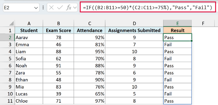
Multiplying the two TRUE/FALSE arrays gives 1 only when both conditions are true, and 0 otherwise. IF reads 1 as TRUE and 0 as FALSE, so you get the same result.
The nice part is that this one formula spills down the column automatically.
Important: The spilling version needs Excel 365 or 2021. On older versions, use the per-row IF with AND formula and copy it down the column.
IF with AND for Three or More Conditions
AND isn’t limited to two conditions, so you can keep adding more inside the same formula. Let’s tighten the pass rule a little.
Below is the same list of students, with the exam score in column B, attendance in column C, and assignments submitted in column D.
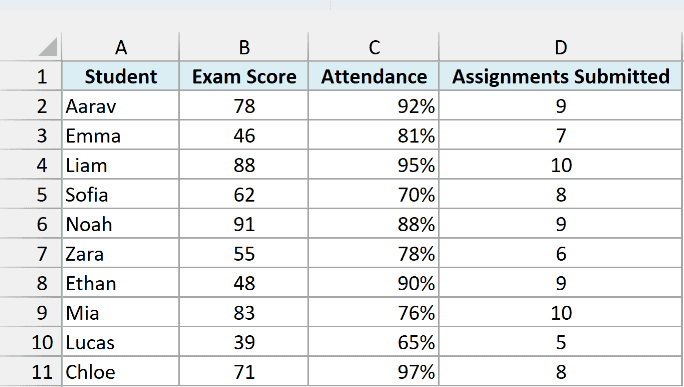
I now want to give a “Pass” only to students who scored at least 50, have at least 75% attendance, and submitted at least 8 assignments. All three have to be true.
Here is the formula:
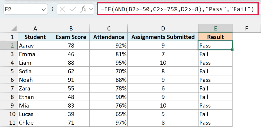
=IF(AND(B2>=50,C2>=75%,D2>=8),"Pass","Fail")
How does this formula work?
I’ve added a third condition, D2>=8, inside the AND function. Now a student only passes when all three conditions are true at the same time.
Notice that Zara no longer passes. Her score and attendance still qualify, but she submitted only 6 assignments, so the whole AND test turns FALSE.
IF with AND to Check If a Value Is Between Two Numbers
A really handy use of IF with AND is checking whether a number falls between a lower and an upper limit.
Below is the same student list. This time, only the exam score in column B matters.
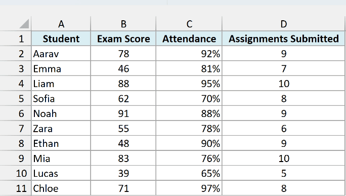
Let’s say students who scored from 45 to 49 (just short of the pass mark) get a chance to retake the exam. I want to mark them “Yes” and everyone else “No”.
Here is the formula:
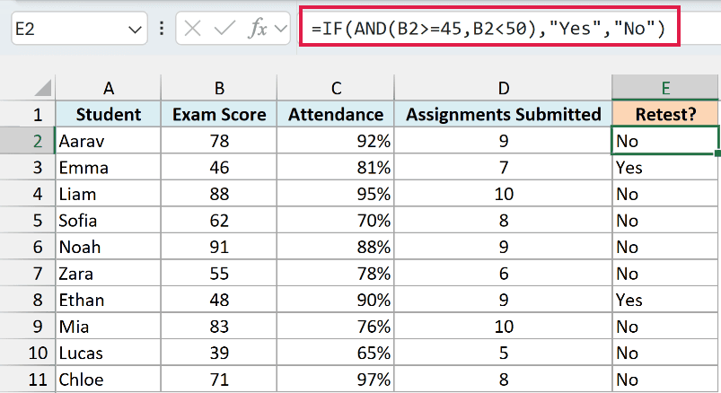
=IF(AND(B2>=45,B2<50),"Yes","No")
How does this formula work?
A single comparison can’t check both limits at once, so AND joins two tests on the same cell. B2>=45 checks the lower limit, and B2<50 checks the upper limit.
Emma (46) and Ethan (48) pass both tests, so they get “Yes”. Lucas (39) is too low and everyone else is 50 or above, so they get “No”.
Pay attention to which comparison you use at each end. Here >= includes 45, while < leaves out 50, since a score of 50 is already a pass.
Nested IF with AND for More Than Two Outcomes
So far the answer has only been one of two values. Sometimes you want more than two outcomes, and that’s where you nest one IF inside another.
Below is the same student list, with the exam score in column B and attendance in column C.
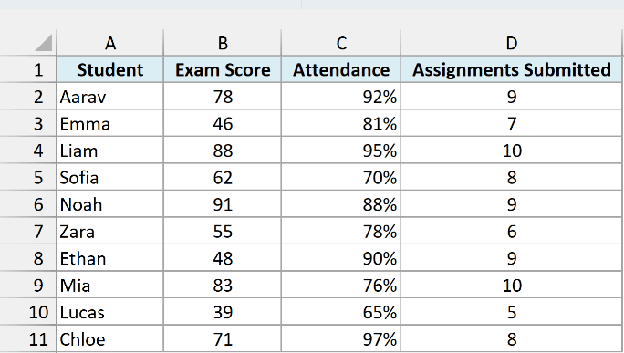
Let’s say students with a score of at least 85 and attendance of at least 90% get “Distinction”.
Students with at least 50 and 75% attendance get “Pass”, and everyone else gets “Fail”.
Here is the formula:
=IF(AND(B2>=85,C2>=90%),"Distinction",IF(AND(B2>=50,C2>=75%),"Pass","Fail"))
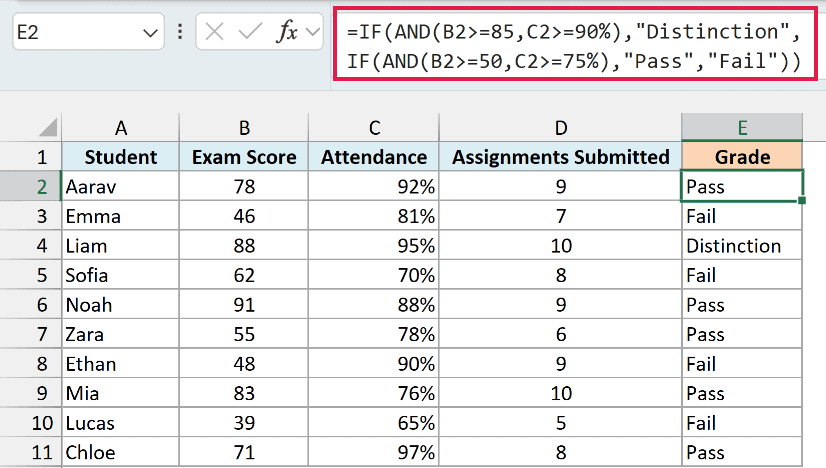
How does this formula work?
The first AND(B2>=85,C2>=90%) checks for a distinction. If that’s true, IF returns “Distinction” and stops.
If it’s false, the second IF runs its own AND(B2>=50,C2>=75%) test. If that’s true it returns “Pass”, and if not it returns “Fail”.
So Liam gets a distinction. Noah scored 91, but his attendance is 88%, so he lands in “Pass” instead.
The order matters here. Always put the strictest test first, because IF stops at the first test that comes back TRUE.
If you’re on Excel 2019, 2021, or Microsoft 365, the IFS function does the same thing with a flatter layout that’s easier to read:
=IFS(AND(B2>=85,C2>=90%),"Distinction",AND(B2>=50,C2>=75%),"Pass",TRUE,"Fail")
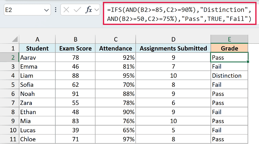
IFS checks each condition in order and returns the value for the first one that’s true.
The final TRUE acts as a catch-all, which is why it returns “Fail” when neither of the earlier tests passes.
Important: IFS is only available in Excel 2019, 2021, and Microsoft 365. On Excel 2016 and older, stick with the nested IF and AND formula shown above.
In this article, I showed you how to combine the IF function with AND to test several conditions at once.
We went from a simple two-condition check all the way to nested formulas with multiple outcomes.
I hope you found this article helpful.
Other Excel Articles You May Also Like:
