

If you want to check several conditions and return a different result for each, the IFS function is what you’re looking for. It runs through your conditions in order and returns the result for the first one that’s true.
It’s the cleaner replacement for stacking a bunch of IF functions inside each other, which gets messy fast. In Excel 365, you can also feed IFS a range and the results spill into the cells below.
The IFS function is available in Excel 2019, 2021, 2024, and Microsoft 365, plus Excel on the web. It’s not in Excel 2016 or earlier, so on those versions you’ll need nested IFs instead.
Follow along with the example file
IFS Function Examples.xlsx
IFS Function Syntax
Here is the syntax of the IFS function:
=IFS(logical_test1, value_if_true1, [logical_test2, value_if_true2], ...)
- logical_test1 – the first condition to check. It has to evaluate to either TRUE or FALSE (like
B2>=90orA2="Yes"). - value_if_true1 – the result you get back when logical_test1 is TRUE.
- [logical_test2, value_if_true2] – optional extra condition-and-result pairs. You can keep adding pairs, up to 127 of them.
The pairs are checked from left to right, and IFS stops at the very first condition that’s TRUE. So the order you list them in matters a lot, which is something I’ll come back to in the examples.
Pro Tip: Every condition needs its own result. If you add a logical_test without a matching value, Excel tells you that you’ve entered too few arguments.
When to Use the IFS Function
Use the IFS function when you need to:
- Sort values into categories, like turning scores into labels or numbers into tiers.
- Check several conditions at once and return a specific answer for each.
- Replace a long, hard-to-read nested IF formula with something flatter and easier to follow.
Let me show you a few practical examples of how the IFS function works.
Example 1: Assign a Status From a Completion Percentage
Let’s start with a simple example.
Below is a small project tracker with the task name in column A and completion in column B, entered as numbers from 0 to 100. For example, 65 means 65% complete. I want a plain-English status for each task.
These formulas use 50, 90, and 100 because the source values use that scale. If you enter actual Excel percentages such as 65%, use percentage cutoffs instead.
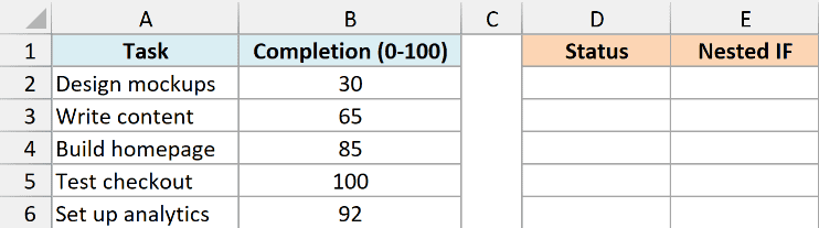
For completion values from 0 to 100, I want anything under 50 to read “Just Started”, anything from 50 to under 90 to read “In Progress”, and 90 through 100 to read “Nearly Done”.
Here is the formula:
=IFS(B2:B6<50,"Just Started",B2:B6<90,"In Progress",B2:B6<=100,"Nearly Done")
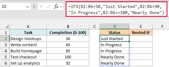
Because I passed the whole range B2:B6 in one go, the formula spills a status down column D automatically. You type it once in D2 and Excel fills the rest, no dragging needed.
IFS checks each row against the conditions in order. A value of 65 fails the first test (under 50), passes the second (under 90), and returns “In Progress”. A value of 100 falls through to the last condition and returns “Nearly Done”.
The order is doing real work here. Since IFS stops at the first TRUE, the “under 90” test only ever sees values that already failed “under 50”, so each band is clean.
Pro Tip: The spilling version works in Microsoft 365, Excel 2021, Excel 2024, and Excel for the web. On Excel 2019, put =IFS(B2<50,”Just Started”,B2<90,”In Progress”,B2<=100,”Nearly Done”) in D2 and copy it down.
Example 2: Pick a Value Between Two Numbers
Here’s a really common use: picking a result based on which number range a value falls into.
Below I have an orders table with the order ID in column A and the package weight in kilograms in column B. I want the shipping cost in column D, based on weight brackets.
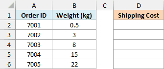
I want to charge 5 for anything under 1 kg, 8 from 1 to under 5 kg, 12 from 5 to under 10 kg, 18 from 10 to under 20 kg, and 25 for anything 20 kg and over.
Here is the formula:
=IFS(B2:B6<1,5,B2:B6<5,8,B2:B6<10,12,B2:B6<20,18,B2:B6>=20,25)
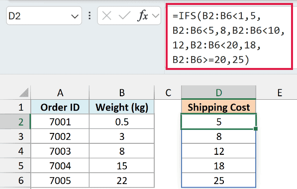
This spills a cost down column D. A 3 kg package fails “under 1” but passes “under 5”, so it costs 8. A 15 kg package lands in the “under 20” bracket and costs 18.
This is the trick for a “between two numbers” lookup. You only ever write the upper edge of each band, because a value that reached the “under 5” test has already been ruled out of “under 1”. IFS handles the lower edge for you.
Keep the conditions in ascending order. If you put a wider test like B2:B6<20 first, every package under 20 kg would match it and get charged 18.
Example 3: Add a Default Value With the TRUE Catch-All
Now let’s handle the case where a value doesn’t match any of your conditions.
Below I have a staff list with the name in column A and a department code in column B. I want the full department name in column D, but some codes are typos or unknown, and I don’t want those to break.
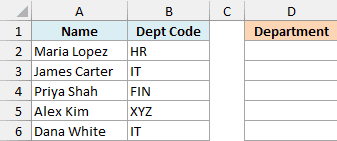
I want “HR”, “IT”, and “FIN” spelled out, and anything else to read “Unknown” instead of throwing an error.
Here is the formula:
=IFS(B2:B6="HR","Human Resources",B2:B6="IT","Information Technology",B2:B6="FIN","Finance",TRUE,"Unknown")
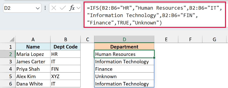
The important part is the TRUE at the end. If none of the real conditions match, IFS reaches TRUE, which is always true, and returns “Unknown”.
Without that catch-all, an unmatched code (like a stray “XYZ”) would return a #N/A error, because IFS needs at least one condition to be TRUE.
Putting TRUE last is the standard way to add an “everything else” result, the same idea as the else in an if-else statement.
Pro Tip: If your conditions test a single value against an exact match like this, the SWITCH function is often tidier. IFS is the better pick the moment you need comparisons like greater-than or less-than.
Example 4: Use IFS With AND for Multiple Conditions
Let’s step it up. Sometimes one branch needs two things to be true at once, and that’s where you nest the AND function inside IFS.
Below is a hiring shortlist with the candidate in column A, their years of experience in column B, and their test score in column C. I want a decision in column D based on both numbers together.
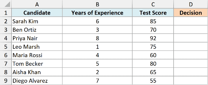
I want “Interview” for anyone with at least 5 years and a score of 80 or more, “Shortlist” for at least 2 years and a score of 65 or more, and “Reject” for everyone else.
Here is the formula:
=IFS(AND(B2>=5,C2>=80),"Interview",AND(B2>=2,C2>=65),"Shortlist",TRUE,"Reject")
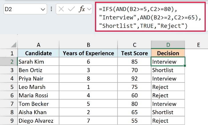
Each AND wraps two conditions, so that branch only fires when both are true. A candidate with 6 years and a score of 85 clears the first AND and gets “Interview”.
Someone with 3 years and a score of 70 fails the first AND but clears the second, so they land on “Shortlist”.
I’m keeping this one as a per-row formula copied down, rather than spilling it over a range. That’s because AND collapses a whole range into a single TRUE or FALSE.
So it can’t test each row on its own inside a spilled formula. Copying the formula down keeps every row honest.
IFS vs Nested IF Statements
Before IFS came along, the way to test several conditions was to stack IF functions inside each other. That still works, but it gets unreadable quickly.
Here is the completion status from Example 1 written the old way. It agrees with IFS for completion values from 0 to 100. Above 100, this IF returns “Nearly Done”, while the IFS formula returns #N/A.
=IF(B2<50,"Just Started",IF(B2<90,"In Progress","Nearly Done"))
Every extra condition means another IF, another comma, and another closing bracket to track at the end. With five or six conditions it turns into a wall of parentheses that’s painful to edit.
IFS flattens all of that into one clean list of condition-and-result pairs. No nesting, no pile of brackets to count. For a straight run of conditions, IFS is almost always the easier one to read and fix later.
Tips & Common Mistakes
A few things to keep in mind so IFS behaves the way you expect:
- A #N/A error means nothing matched. If none of your conditions are TRUE, IFS returns #N/A. Add a final
TRUEwith a default result (as in Example 3) to catch everything else. - Order your conditions carefully. IFS stops at the first TRUE, so a broad condition placed too early can shadow a narrower one below it. For number ranges, list them from smallest to largest.
- Every test needs a result. Conditions and results come in pairs. A lone logical_test with no value gives you a “too few arguments” error.
- A #VALUE! error means a test didn’t return TRUE or FALSE. Each logical_test has to resolve to a real TRUE or FALSE. Check for a stray reference or a typo in that condition.
- Not on Excel 2019 or later? IFS doesn’t exist in Excel 2016 or earlier. On those versions, fall back to nested IFs or look them up another way.
Wrapping Up
The IFS function is one of those small upgrades that makes your formulas a lot easier to live with. Line up your conditions, remember they’re checked in order, and drop a TRUE at the end whenever you want a fallback.
I hope you found this tutorial helpful. If you get stuck on an IFS formula, it usually comes down to condition order or a missing default.
Other Excel Articles You May Also Like:
