

If you want to quickly find out how many rows are in a range, a table, or the result of a formula, the ROWS function is what you’re looking for.
ROWS returns a single number, but it works nicely inside dynamic array formulas like =SEQUENCE(ROWS(A2:A13)) to build a spilled list of numbers.
In this article, I’ll show you how to use the ROWS function with practical examples, from a simple row count to numbering a list and counting records that match a condition.
ROWS Syntax
Here is the syntax of the ROWS function:
=ROWS(array)
- array – The array, array formula, or range of cells you want to count the rows in. This is the only argument, and it is required.
The function returns one number: the count of rows in whatever you hand it.
One thing worth clearing up early. ROWS (with an S) counts how many rows are in a range. ROW (no S) returns the row number of a single cell. They sound alike but do different jobs, and mixing them up is the most common ROWS mistake.
When to Use the ROWS Function in Excel
Use the ROWS function when you need to:
- Count how many rows a range or table holds without selecting it and reading the status bar
- Feed a row count into another function, like SEQUENCE to number a list
- Count how many records a formula like FILTER returns
- Size a reference so a formula always points at the last row, even as data grows
Let me show you a few practical examples of how this works.
Example 1: Count the Number of Rows in a Range
Let’s start with a simple example.
Below is a dataset of support tickets. Column A has the ticket ID, column B the customer, column C the priority, and column D the status. The data sits in rows 2 to 13.
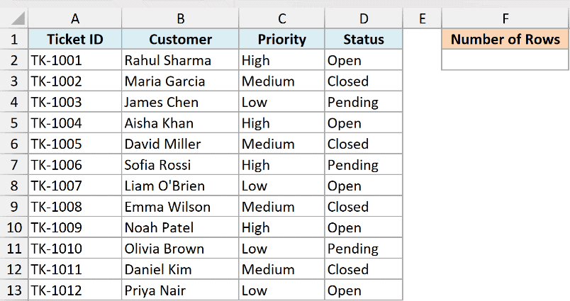
I want to know how many tickets are in this list without manually selecting the range.
Here is the formula:
=ROWS(A2:A13)
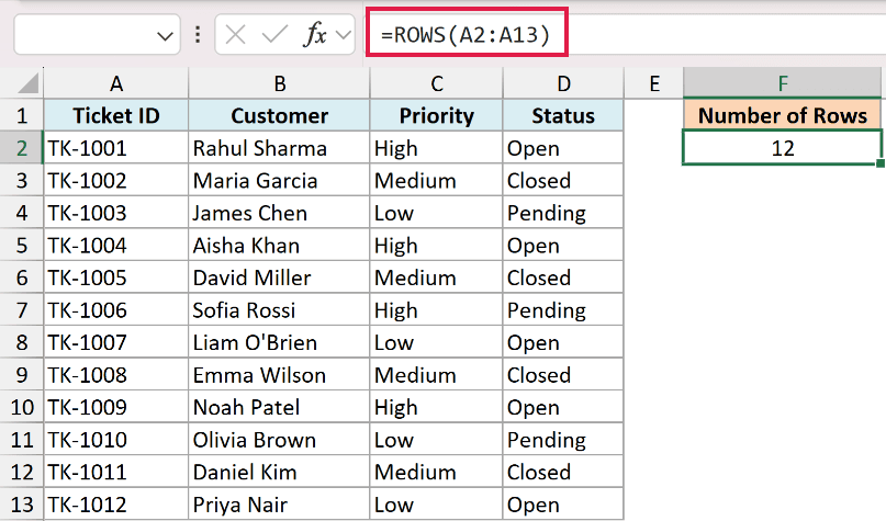
The range A2:A13 spans 12 rows, so ROWS returns 12. That matches the 12 tickets in the list.
A common mix-up is expecting this to count cells. It does not. Even =ROWS(A2:D13) returns 12, because ROWS counts rows, not cells, no matter how many columns the range covers.
Example 2: Count the Rows in an Excel Table
Here’s a more practical scenario.
The same ticket data is now formatted as an Excel Table named Tickets. The nice thing about a Table is that it grows on its own as you add new tickets below it.
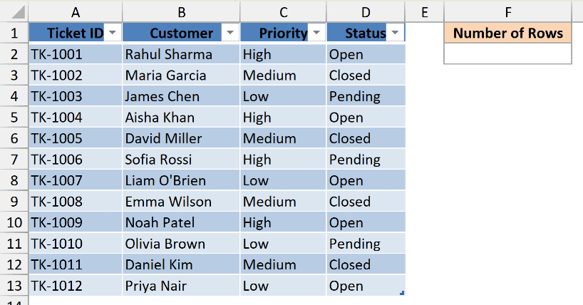
I want a live count of tickets that updates automatically whenever a new row is added to the Table.
Here is the formula:
=ROWS(Tickets)
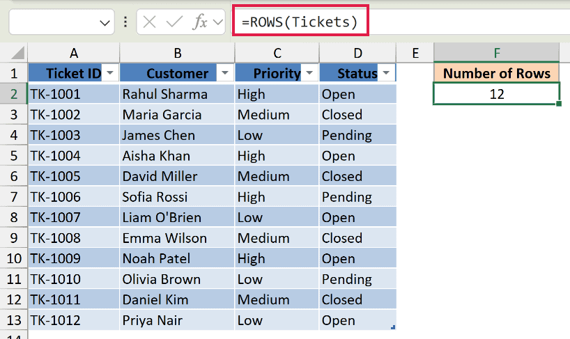
The Table has 12 data rows, so this returns 12. Since the reference points at the Table itself, adding a 13th ticket pushes the count to 13 with no formula edit.
Pro Tip: ROWS on a Table counts the data rows only. The header row is not included, so you get a clean record count.
Example 3: Add Serial Numbers That Spill Automatically
Now let’s use ROWS inside another function.
I have the same list of customers in column B, rows 2 to 13, and I want a serial number next to each one.
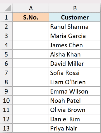
I want a single formula that fills the whole serial-number column, from 1 down to however many customers there are.
Here is the formula:
=SEQUENCE(ROWS(B2:B13))
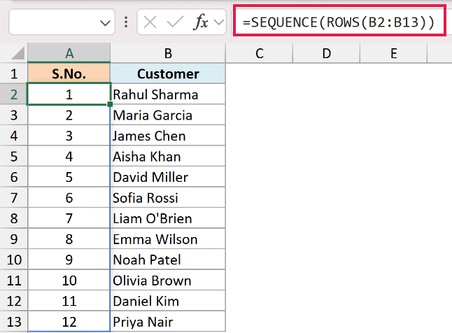
Here, ROWS counts the customers (12) and hands that number to SEQUENCE, which spills the numbers 1 to 12 down the column. You enter it once and the results fill the cells below automatically.
The advantage over typing numbers by hand is that the count drives the length. Point ROWS at a bigger range and the serial list grows to match, with no dragging.
Pro Tip: On Excel versions without SEQUENCE, put =ROWS($B$2:B2) in the first cell and fill it down. The range expands as you go, so each cell counts one more row than the last: 1, 2, 3, and so on.
Example 4: Count Records That Match a Condition
Let’s step it up with something I use quite often.
Back to the ticket dataset in rows 2 to 13, with the priority in column C. I want to know how many tickets are marked High priority.
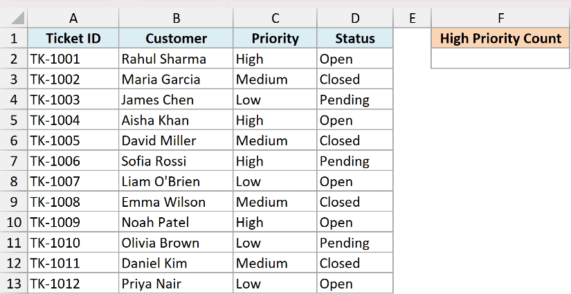
I want ROWS to count the rows that FILTER returns, so I get the number of High-priority tickets.
Here is the formula:
=ROWS(FILTER(A2:A13,C2:C13="High"))
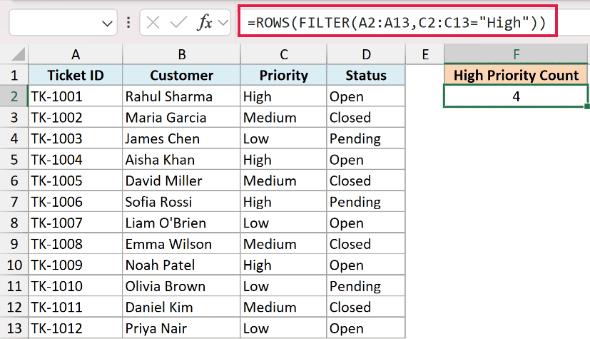
How this formula works:
- FILTER pulls only the ticket IDs where the priority in column C equals “High”, which is 4 of them
- ROWS then counts the rows in that filtered result and returns 4
This is the dynamic-array side of ROWS. It does not spill on its own, but it happily counts the array another function produces. FILTER is available in Excel 365 and Excel 2021.
Pro Tip: If no rows match, FILTER returns an error and so does ROWS. Wrap it as =IFERROR(ROWS(FILTER(A2:A13,C2:C13=”High”)),0) to show 0 instead.
Example 5: Return the Last Value in a List
Here’s a handy trick that uses ROWS to always land on the last row.
I have the list of customers in column A, rows 2 to 13, and I want to pull the customer from the very last row without knowing its position.
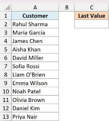
I want the last customer name in the list, and I want it to keep working even if I add or remove rows later.
Here is the formula:
=INDEX(A2:A13,ROWS(A2:A13))
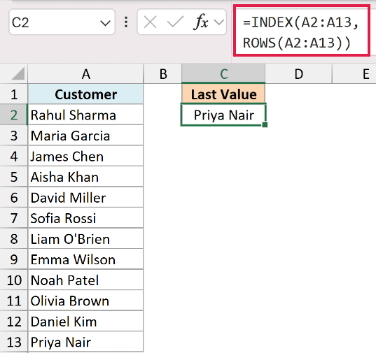
Here, ROWS(A2:A13) returns 12, and INDEX returns the value in the 12th position of the range, which is the last customer, Priya Nair.
Because ROWS recalculates the count every time, the formula always points at the final row. If the list shrinks to 10 rows, ROWS returns 10 and INDEX follows along.
Example 6: Check That Two Lists Have the Same Number of Rows
Let’s finish with a quick validation check.
I have two lists I want to compare before merging them. The first list is in A2:A13 and the second is in C2:C15. I want to be sure they have the same number of rows first.
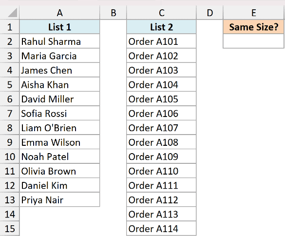
I want a TRUE or FALSE that tells me whether both lists are the same length.
Here is the formula:
=ROWS(A2:A13)=ROWS(C2:C15)
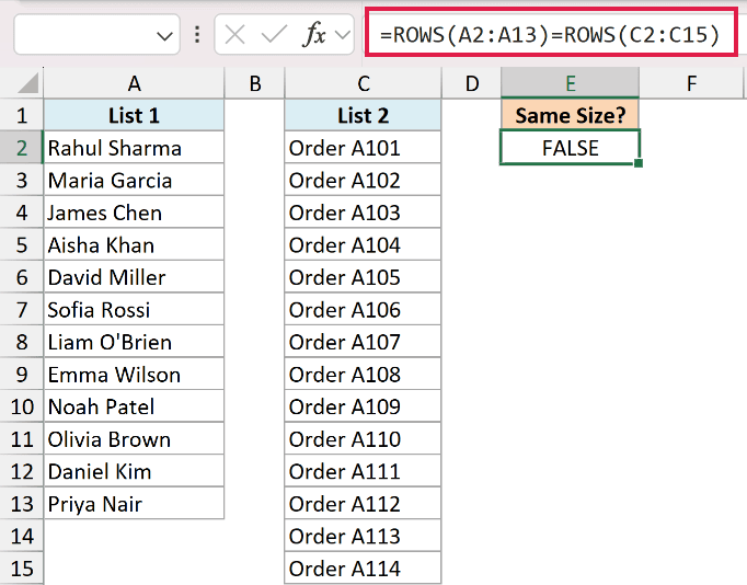
The first range has 12 rows and the second has 14, so the two counts do not match and the formula returns FALSE.
This is a fast sanity check before you line two imports up side by side. A FALSE tells you one list is missing rows before a bad comparison ever happens.
Tips & Common Mistakes
- ROWS vs ROW: ROWS counts how many rows are in a range. ROW returns the row number of a single cell. If a formula gives an unexpected count of 1, check whether you meant ROWS.
- It counts rows, not cells: ROWS(A2:D13) returns 12, not 48. The number of columns never changes the answer. Use COLUMNS if you want the column count instead.
- Blank rows still count: ROWS counts every row in the range you give it, empty or not. If you only want rows with data, use COUNTA or a filtered count instead.
- Point at a Table or a spilled range to stay dynamic: ROWS(Tickets) or ROWS(A2#) both update on their own as the data grows, so you avoid hard-coded ranges.
- One argument only: ROWS takes a single range or array. If you need to add up counts from separate ranges, wrap each in its own ROWS and add them.
The ROWS function looks simple, and it is, but it earns its place once you start nesting it. It sizes serial-number lists, counts the results of a FILTER, and points formulas at the last row without you tracking the count by hand.
Keep the ROW-versus-ROWS distinction in mind and you’ll reach for the right one every time.
Other Excel Articles You May Also Like:
