

If you want to pull a value from a specific spot in a table, based on its row and column position, the INDEX function is what you’re looking for. You tell it a range and a position, and it hands back the value sitting there.
On its own it’s simple, but INDEX really shines when you pair it with MATCH to build lookups that VLOOKUP can’t handle. In Excel 365, INDEX can also return an entire row or column at once, spilling those values into the cells below.
In this article, I’ll show you how to use INDEX in Excel, from a basic position lookup to two-way lookups, left lookups, drop-down dashboards, three-way lookups, and dynamic ranges.
INDEX Syntax
INDEX has two forms. The one you’ll use most is the array form:
=INDEX(array, row_num, [column_num])
- array – the range of cells you want to pull a value from.
- row_num – the row position within the range (the first row is 1).
- column_num – optional. The column position within the range. You can skip it if the range is a single column or row.
The second form is the reference form, which lets you point at more than one range and pick between them:
=INDEX(reference, row_num, [column_num], [area_num])
Here reference can be several ranges, and area_num tells INDEX which of those ranges to use (see the three-way lookup in Example 7). This form also returns a cell reference, not just a value, which is handy for building dynamic ranges (see Example 8).
Pro Tip: If you set row_num or column_num to 0, INDEX returns the whole column or row instead of a single value. In Excel 365 that result spills into the neighboring cells.
INDEX works in every version of Excel, from Microsoft 365 and Excel 2024 back to the older ones, plus Excel on the web.
When to Use the INDEX Function
Use INDEX when you need to:
- Grab a value from a known row and column position in a range.
- Build a lookup with MATCH that can search in any direction, including to the left.
- Do a two-way lookup that matches both a row and a column at once, or drive it from drop-down lists.
- Do a three-way lookup that also picks between multiple tables.
- Return a whole row or column, aggregate it with SUM or MAX, or set a dynamic range endpoint.
Let me show you a few practical examples of how INDEX works.
Example 1: Get a Value by Its Position
Let’s start with the simplest case: pulling a value from a known position in a grid.
Below is a small price grid for a coffee shop. Column A has the drink names, and columns B, C, and D hold the prices for the Small, Medium, and Large sizes.
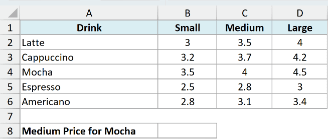
I want the Medium price for Mocha, which sits in the third row and second column of the price block B2:D6.
Here is the formula:
=INDEX(B2:D6,3,2)
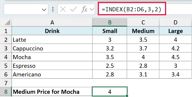
This returns 4.
INDEX looks inside the range B2:D6, counts down to the third row (Mocha), then across to the second column (Medium), and returns the value it finds there. The positions are counted from the top-left of the range, not from the worksheet’s row and column numbers.
Example 2: Return an Entire Column or Row
Now let’s use INDEX to pull back a whole column or a whole row at once, instead of a single cell.
Below is a sales table. Column A has the salespeople, and columns B through E hold their Q1 to Q4 sales figures.
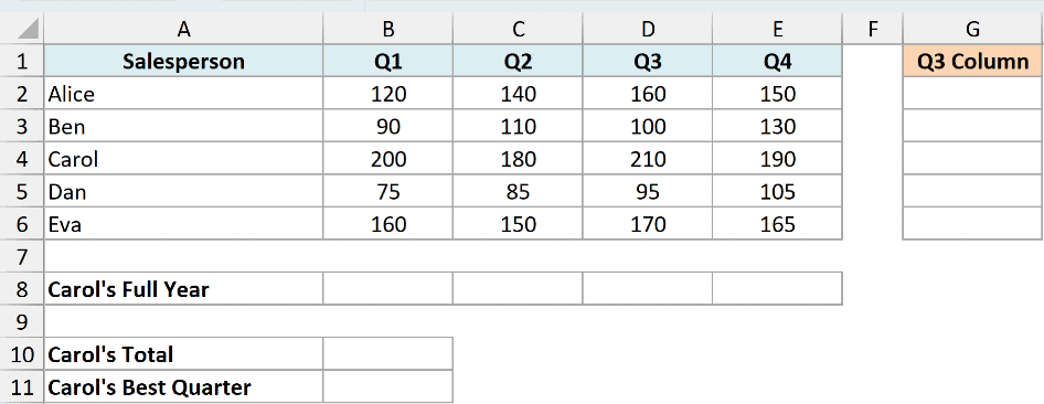
First, I want all of the Q3 figures, which is the third column of the range B2:E6.
Here is the formula:
=INDEX(B2:E6,0,3)
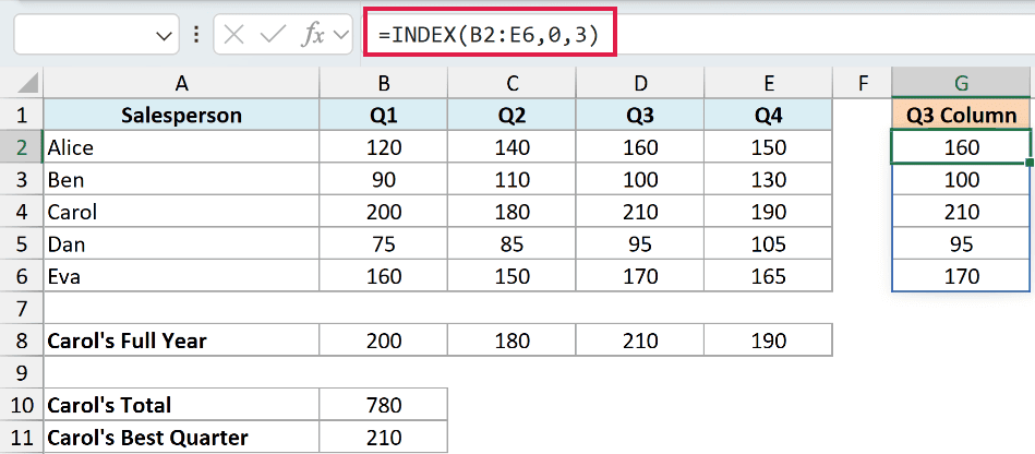
The 0 for row_num tells INDEX to ignore the row and return the entire third column. In Excel 365 those five values spill down the cells below the formula.
Now let’s do the same thing for a row. I want Carol’s full year, which is the third row of the range.
Here is the formula:
=INDEX(B2:E6,3,0)
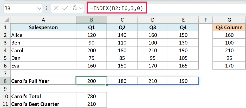
This time the 0 goes in the column_num spot, so INDEX returns the whole third row (Carol’s four quarters), spilling them across to the right.
Pro Tip: The spilling behavior needs Microsoft 365 or Excel for the web. On Excel 2019 or earlier, you’d select the output cells first and confirm the formula with Ctrl + Shift + Enter.
Because INDEX(...,0) hands back the whole row as an array, you can wrap it in a function like SUM, MAX, or MIN to aggregate it in a single formula.
Let’s say I want Carol’s total sales for the year.
Here is the formula:
=SUM(INDEX(B2:E6,3,0))
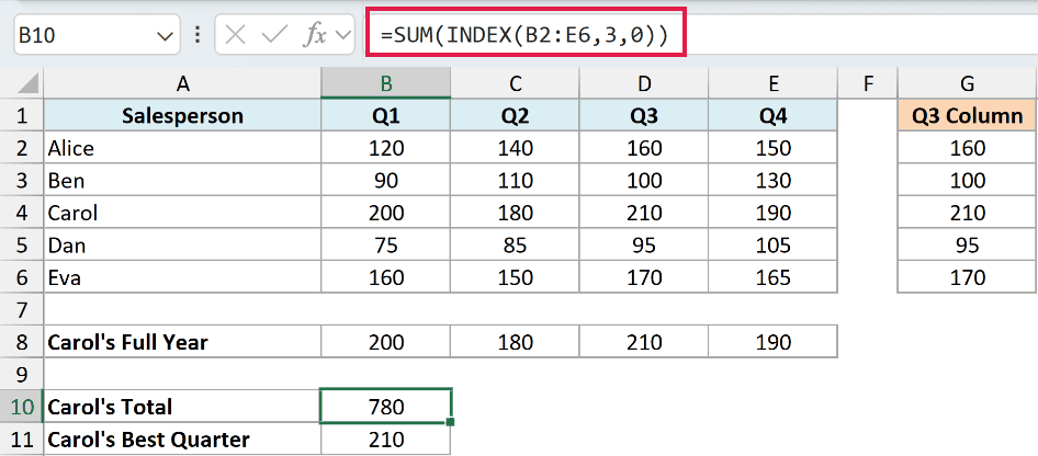
This returns 780.
INDEX returns Carol’s four quarters as an array, and SUM adds them up. No helper column and no need to point at B4:E4 by hand.
Now let’s find her best quarter instead.
Here is the formula:
=MAX(INDEX(B2:E6,3,0))
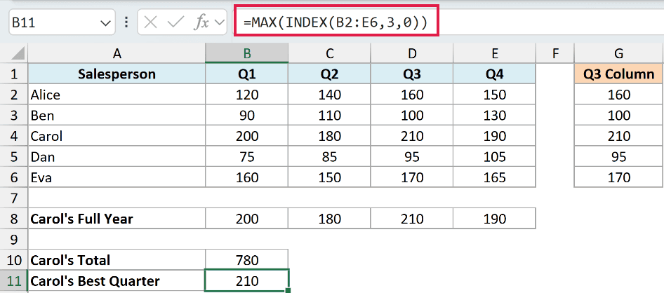
This returns 210. Swap MAX for MIN to get her weakest quarter, or for AVERAGE to get her quarterly average.
Example 3: INDEX and MATCH for a One-Way Lookup
INDEX gets really useful once you stop typing the position by hand and let the MATCH function find it for you. This is the classic INDEX and MATCH lookup.
Below is a product list, with the product name in column A and its price in column B.
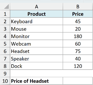
I want the price of the Headset without counting rows myself.
Here is the formula:
=INDEX(B2:B8,MATCH("Headset",A2:A8,0))
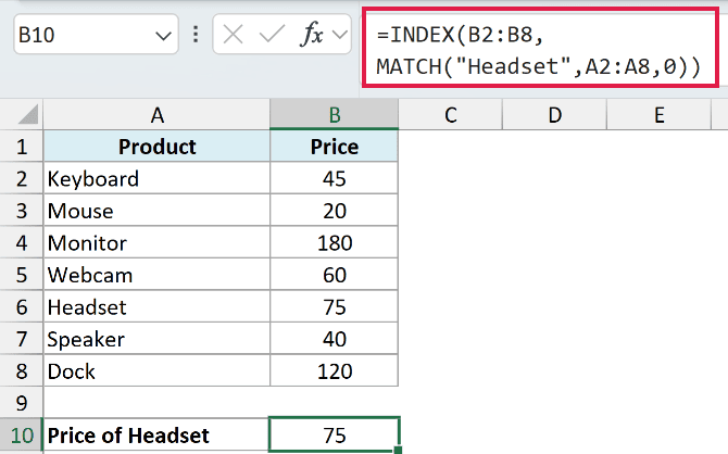
This returns 75.
Here MATCH looks down A2:A8, finds “Headset” in the fifth position, and passes that 5 to INDEX as the row number. INDEX then returns the fifth price from B2:B8. Change the name and the price updates on its own.
Pro Tip: For a plain one-way lookup like this on Excel 365 or 2021, the XLOOKUP function is cleaner. INDEX and MATCH still wins for two-way lookups and dynamic ranges, and it works in every version of Excel.
Example 4: Left Lookup Where VLOOKUP Can’t Reach
Here’s the big reason people learn INDEX and MATCH: it can look to the left. VLOOKUP can only return a value from a column to the right of the one it searches, but INDEX doesn’t care about direction.
Below is an employee table. The name is in column A, the department in column B, and the employee ID in column C.
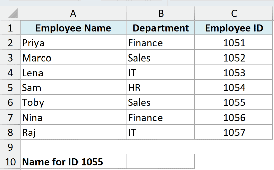
I have an employee ID (1055) and I want the name, which sits to the left of the ID column.
Here is the formula:
=INDEX(A2:A8,MATCH(1055,C2:C8,0))
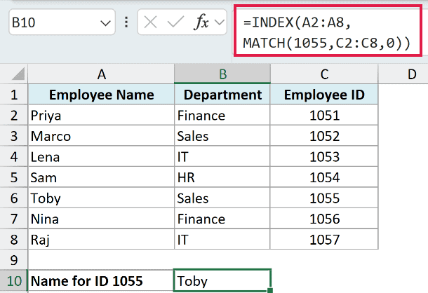
This returns Toby.
MATCH finds 1055 in the fifth position of the ID column C2:C8, and INDEX returns the fifth name from column A. The lookup column (C) is to the right of the answer column (A), which VLOOKUP simply can’t do.
Example 5: Two-Way Lookup with INDEX and MATCH
Now let’s match a row and a column at the same time. This is called a two-way lookup, and it uses MATCH twice: once for the row and once for the column.
Below is a sales grid. The products run down column A, the regions run across the top row, and the sales figures fill the middle.
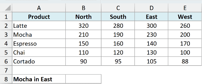
I want the sales figure for Mocha in the East region, where the row and the column meet.
Here is the formula:
=INDEX(B2:E6,MATCH("Mocha",A2:A6,0),MATCH("East",B1:E1,0))
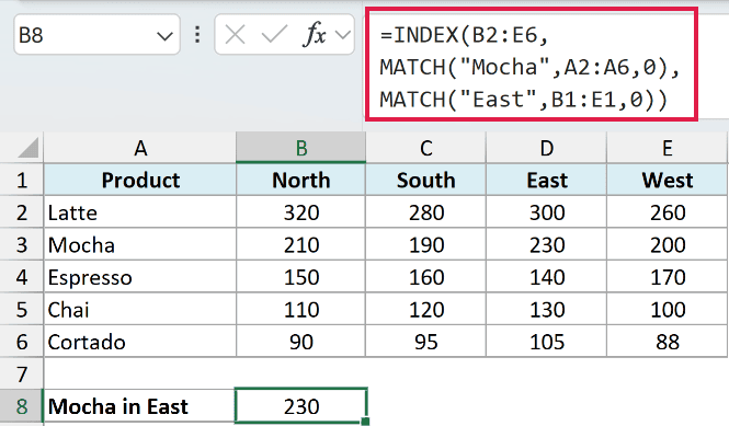
This returns 230.
The first MATCH finds “Mocha” down the product column (position 2), and the second MATCH finds “East” across the region row (position 3). INDEX then returns the value where row 2 and column 3 cross inside B2:E6. Change either lookup and the result follows.
Example 6: Run a Two-Way Lookup from Drop-Down Lists
Typing the lookup names by hand gets tedious and invites typos. A nicer setup is to pick them from drop-down lists, so the result updates the moment you change a selection. This makes a neat little dashboard.
Below is a scores table. The students run down column A, the subjects run across row 1, and the marks fill the grid B2:E5.
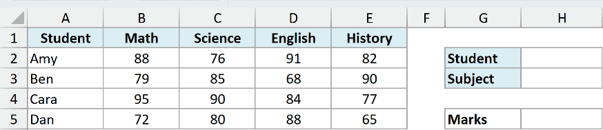
I want to pick a student in cell H2 and a subject in cell H3 from drop-downs, and see that student’s mark for that subject.
First, set up the two drop-downs. Select cell H2, go to Data > Data Validation, choose List under Allow, set the source to A2:A5 (the student names), and click OK.
Repeat for cell H3, this time pointing the source at B1:E1 (the subject names).
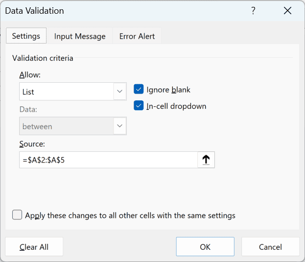
Now the same two-way INDEX and MATCH formula reads its lookup values from those two cells.
Here is the formula:
=INDEX(B2:E5,MATCH(H2,A2:A5,0),MATCH(H3,B1:E1,0))
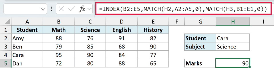
With Cara and Science selected, this returns 90.
MATCH turns the student in H2 into a row number and the subject in H3 into a column number, and INDEX returns the mark where they cross. Change either drop-down and the result follows instantly.
Pro Tip: Behind a small on-screen grid you can keep a table of hundreds of students. The reader only touches the two drop-downs, which makes this a handy dashboard component for a report.
Example 7: Three-Way Lookup with the Reference Form
Here’s where the reference form of INDEX earns its keep. On top of a row and a column, it can pick between several tables using the area_num argument, which gives you a three-way lookup.
Below are three score tables stacked in the same columns, one per term. Each has the same students down column A and the same subjects across the top: Term 1 in B2:D4, Term 2 in B7:D9, and Term 3 in B12:D14.
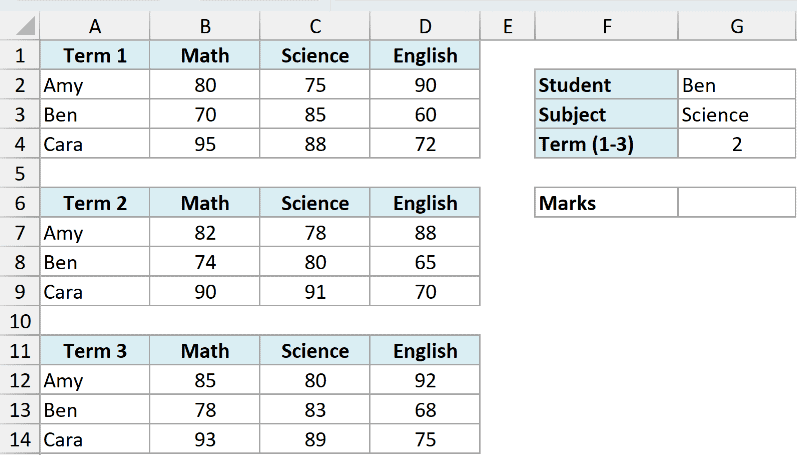
I want to pick a student, a subject, and a term, and get that one mark. I’ve put the student in G2, the subject in G3, and the term number (1, 2, or 3) in G4.
Here is the formula:
=INDEX((B2:D4,B7:D9,B12:D14),MATCH(G2,A2:A4,0),MATCH(G3,B1:D1,0),G4)
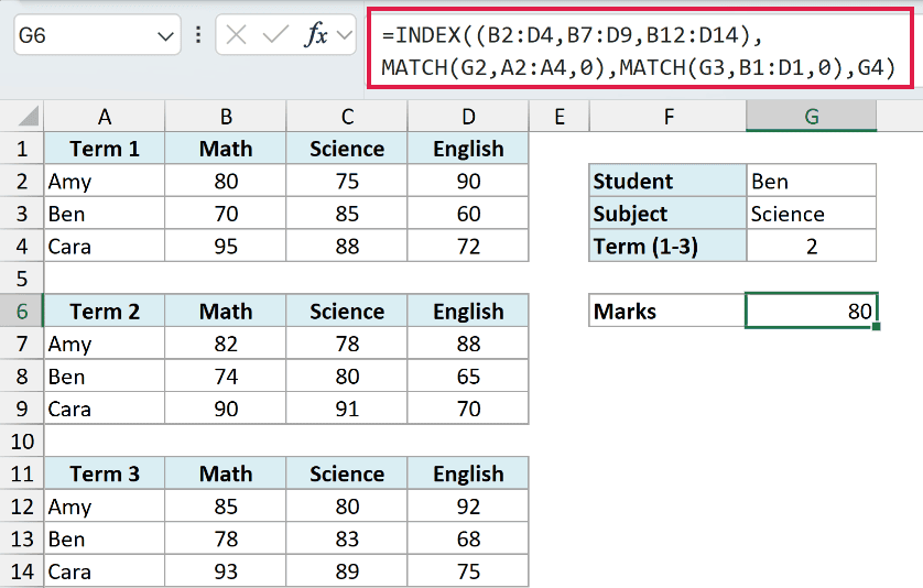
With Ben, Science, and term 2 selected, this returns 80.
How this formula works:
- The three ranges in parentheses
(B2:D4,B7:D9,B12:D14)are the reference. This is what tells INDEX to expect an area_num. - MATCH(G2,A2:A4,0) finds Ben’s row position (2), and MATCH(G3,B1:D1,0) finds Science’s column position (2). The students and subjects line up across all three tables, so one MATCH each is enough.
- G4 is the area_num. A 2 tells INDEX to look inside the second range, Term 2, and return the value where row 2 and column 2 meet.
Pro Tip: If you’d rather pick a term name than a number, hold the labels somewhere and swap G4 for a MATCH that turns the name into 1, 2, or 3. Wrap the whole thing in a drop-down for each input and you have a three-way dashboard.
Example 8: Build a Dynamic Range with INDEX
This one uses the fact that INDEX returns a cell reference, not just a value. That lets you use it as one end of a range, so the range can grow or shrink on its own.
Below is a monthly sales table, with the month in column A and the sales amount in column B for all twelve months.
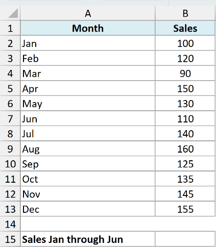
I want to add up the sales from January through June, which is the first six months.
Here is the formula:
=SUM(B2:INDEX(B2:B13,6))
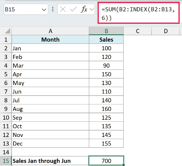
This returns 700.
Here INDEX(B2:B13,6) returns a reference to the sixth cell (B7), not the value inside it. So B2:INDEX(…) becomes the range B2:B7, and SUM adds those six months. Swap the 6 for another number, or point it at a cell, and the range end moves automatically.
Example 9: Pull an Entire Record with INDEX and MATCH
Let’s combine the row-return trick from Example 2 with MATCH to grab a full record in one formula.
Below is an orders table. Column A has the order ID, and the rest of the columns hold the customer, product, quantity, and total.
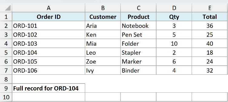
I want the entire row of details for order ORD-104, without knowing which row it’s on.
Here is the formula:
=INDEX(A2:E7,MATCH("ORD-104",A2:A7,0),0)
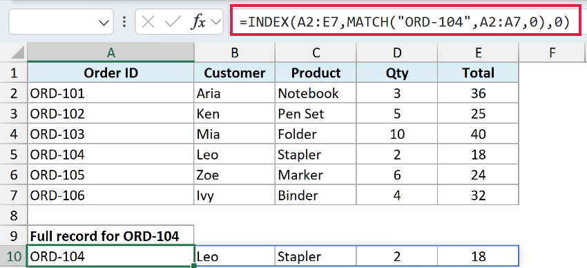
MATCH finds ORD-104 in the fourth position of column A, so INDEX pulls the fourth row.
The 0 in the column_num spot tells INDEX to return the whole row, so all five fields for that order spill across the cells to the right in Excel 365.
Tips & Common Mistakes
A few things to keep in mind when working with INDEX:
- Positions are counted inside the range, not the sheet. In
=INDEX(B2:D6,3,2), row 3 and column 2 are counted from the top-left corner of B2:D6, not from the worksheet’s rows and columns. - INDEX doesn’t error on its own, MATCH does. If a lookup fails, it’s usually MATCH returning #N/A because the value isn’t in the range. Check for typos, extra spaces, or numbers stored as text.
- A #REF! error means the position is out of range. Asking for row 8 in a range that’s only 6 rows tall returns #REF!. Keep row_num and column_num inside the range.
- Use 0 to return a whole row or column. Set row_num to 0 for a full column, or column_num to 0 for a full row. In older Excel you confirm these with Ctrl + Shift + Enter.
- INDEX and MATCH beats VLOOKUP for left lookups. Because INDEX can return from any column, the INDEX and MATCH combo handles lookups to the left, which VLOOKUP can’t.
Wrapping Up
INDEX is a small function that does a lot once it clicks. On its own it returns a value at a given position, and paired with MATCH it powers flexible lookups that reach in any direction, run two-way and three-way tables, drive drop-down dashboards, and build ranges that adjust themselves.
Start with a plain position lookup, then layer in MATCH as your lookups get trickier. I hope you found this tutorial helpful.
Other Excel Articles You May Also Like:
