

If you want to pull the last few characters from a text string in Excel, like the last four digits of a card number or the extension from a file name, the RIGHT function is what you need.
It gives you the characters from the end of the text, and you decide how many you want.
In Excel 365, you can also hand RIGHT a whole range and the results spill into the cells below. In this article, I’ll show you how to use the RIGHT function with a bunch of practical examples.
RIGHT Function Syntax
Here is the syntax of the RIGHT function:
=RIGHT(text, [num_chars])
- text – the text string you want to pull characters from. This can be text in quotes or a reference to a cell.
- num_chars – (optional) how many characters to grab from the end of the text. If you leave this out, RIGHT returns just the last one character.
RIGHT works in every version of Excel, including Microsoft 365, Excel 2024, 2021, 2019, and older, as well as Excel on the web and Mac. The spilling behavior shown in Example 1 needs Excel 365 or 2021.
When to Use the RIGHT Function
Use RIGHT when you need to:
- Pull the last few characters from a value (a suffix, a code, the last four digits of a card).
- Grab everything after a delimiter when you pair it with LEN and FIND.
- Extract a file extension or an email domain.
- Turn trailing text digits into a real number by wrapping it in VALUE.
Let me show you how this works with a few practical examples.
Example 1: Extract the Last Few Characters
Let’s start with the simplest case.
Below I have a list of loyalty card numbers in column A. Each one is a long string of digits, and I only want the last four of each.
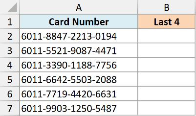
I want to grab the last four characters from every card number in one go.
Here is the formula:
=RIGHT(A2:A7, 4)
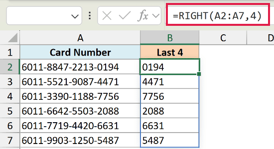
I typed this once in cell B2 and the results spilled down through B7, one last-four for each card. That is dynamic arrays at work.
RIGHT looks at each value, counts four characters in from the right, and returns them. Since I pointed it at the whole range A2:A7, Excel handed back a result for every row.
Pro Tip: On Excel 2019 or older, the range version won’t spill. Just write =RIGHT(A2, 4) in the first cell and copy it down the column instead.
Example 2: Extract a File Extension
Here’s another handy one.
Below I have a list of file names in column A. Each name ends in a three-letter extension like pdf or csv, and I want to pull just that extension out.
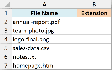
I want the extension from each file name, without the dot.
Here is the formula:
=RIGHT(A2:A7, 3)
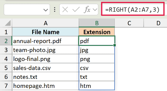
Since every extension here is exactly three characters, asking RIGHT for the last three does the job, and the results spill down the column.
This shortcut only works when the extension is a fixed length. If your list mixes three and four-letter extensions like csv and xlsx, hard-coding a number breaks. For that, you want the dynamic approach in the next example.
Example 3: Extract Text After a Delimiter with LEN and FIND
Now let’s tackle the case where the piece you want isn’t a fixed length.
Below I have full names in column A, first name and last name separated by a space. I want the last name, but last names are all different lengths, so a plain number won’t work.
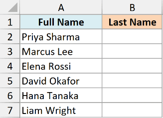
I want to pull out just the last name from each full name.
Here is the formula:
=RIGHT(A2, LEN(A2)-FIND(" ", A2))
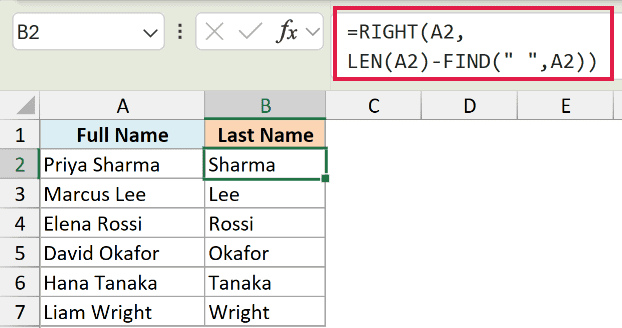
How this formula works:
- FIND(” “, A2) finds the position of the space. For “Priya Sharma” that’s 6.
- LEN(A2) gives the total length of the text, which is 12 here.
- LEN(A2) – FIND(” “, A2) works out how many characters sit after the space, so 12 minus 6 is 6.
- RIGHT then pulls that many characters from the end, giving you “Sharma”.
Because the num_chars is calculated for each row, this handles last names of any length. Copy it down and every row gets the right cut.
Pro Tip: The same formula grabs an email domain if you swap the space for “@”. Use =RIGHT(A2, LEN(A2)-FIND(“@”, A2)) and it returns everything after the @ sign.
In Excel 365 you can also point this whole formula at a range with =RIGHT(A2:A7, LEN(A2:A7)-FIND(” “, A2:A7)) and it spills down for you.
Example 4: Turn Trailing Digits Into a Real Number
This one clears up a common surprise with RIGHT.
Below I have order codes in column A, each ending in a four-digit number. I want those trailing digits as an actual number I can add up or sort.
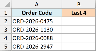
First, let me just pull the last four characters and see what I get.
Here is the formula:
=RIGHT(A2, 4)
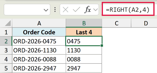
This returns “0475”, but notice it sits on the left of the cell. That’s because RIGHT always gives back text, even when the characters are all digits.
To get a real number, wrap the whole thing in the VALUE function.
Here is the formula:
=VALUE(RIGHT(A2, 4))
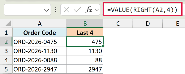
Now the result is 475, sitting on the right of the cell as a proper number. VALUE converts the text digits into a number you can use in calculations. The leading zero drops off, which is expected once it’s a number.
Example 5: Mask an Account Number Showing Only the Last 4
Here’s a practical formatting job.
Below I have full account numbers in column A. I want to hide most of each one and show only the last four digits, the way receipts and websites do.
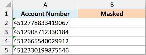
I want to display each account as asterisks followed by its last four digits.
Here is the formula:
="**** **** **** "&RIGHT(A2, 4)
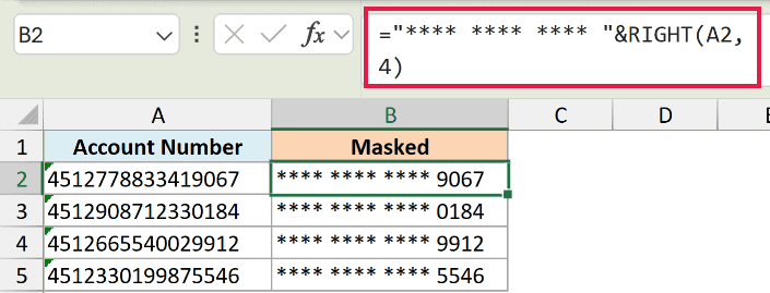
Here, RIGHT pulls the last four digits, and the ampersand (&) joins them onto a block of asterisks. So a full account number turns into something like **** **** **** 9067, hiding everything but the last four.
Pro Tip: Long card numbers should be stored as text, not numbers. Excel only keeps 15 digits of precision, so a 16-digit number stored as a number loses its last digit before RIGHT even sees it.
Example 6: Fix Wrong Results Caused by Trailing Spaces
This last one is a gotcha worth knowing about.
Below I have product codes in column A that were pasted in from another system, and some of them have a stray space at the end. I want the last four characters of each code.
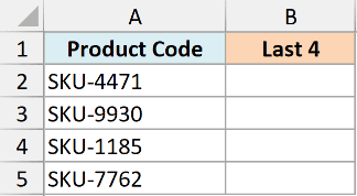
Let me start with the straightforward formula and see what happens.
Here is the formula:
=RIGHT(A2, 4)
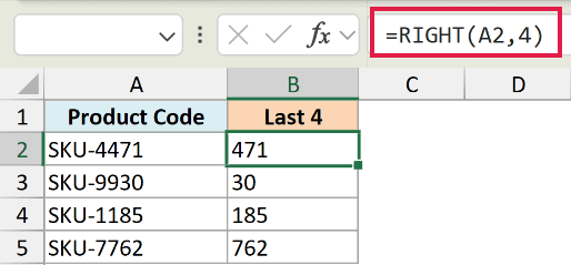
Instead of “4471”, the result comes back as “471 ” with a space on the end. RIGHT counted the trailing space as one of the last four characters, so it grabbed one real character too few.
The fix is to clean the text with TRIM before RIGHT looks at it.
Here is the formula:
=RIGHT(TRIM(A2), 4)
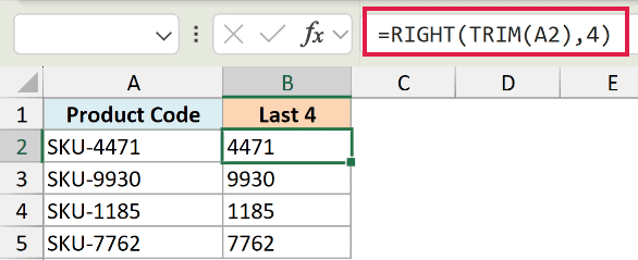
TRIM strips the extra space off the end first, so RIGHT now sees “SKU-4471” and returns a clean “4471”. Whenever your data comes from a copy-paste or an export, wrapping the text in TRIM saves you from these silent errors.
Tips & Common Mistakes
- RIGHT always returns text. Even when the result is all digits, it comes back as text. Wrap it in VALUE when you need a number for math or sorting.
- num_chars must be zero or more. A negative number gives a #VALUE! error. This is the “num_chars must be greater than or equal to zero” message people run into.
- num_chars of 0 returns nothing. RIGHT with a num_chars of 0 gives back an empty string, not an error. Leaving num_chars out entirely returns just the last one character.
- A num_chars bigger than the text is fine. If you ask for more characters than the string has, RIGHT just returns the whole string. No error.
- Watch for trailing spaces. Stray spaces at the end throw the count off. Wrap the text in TRIM when the data comes from an export or copy-paste.
- FIND finds the first match only. In the last-name example, FIND(” “) stops at the first space, so names with a middle name need you to first find the position of the last occurrence of that character. Also remember FIND is case-sensitive while SEARCH is not.
- RIGHT can’t read date parts. A date is really a serial number underneath, so RIGHT won’t pull “2026” out of a real date. Use YEAR, MONTH, and DAY, or the TEXT function, for that.
Conclusion
The RIGHT function is a simple way to pull characters off the end of a text string, and it gets a lot more useful the moment you pair it with LEN, FIND, VALUE, and TRIM.
We covered extracting a fixed number of characters, grabbing text after a delimiter, converting trailing digits into numbers, masking account numbers, and cleaning up trailing spaces. With these patterns, you can handle most real-world text cleanup that involves the end of a string.
For other ways to pull pieces out of your data, take a look at how to extract a substring in Excel.
Other Excel Articles You May Also Like:
