

If you want to pull the first few characters out of a text string in Excel, like a prefix code or the start of a name, the LEFT function is what you’re looking for.
You hand it some text and tell it how many characters to grab, and it returns that many characters from the left side.
In Excel 365, you can also feed LEFT a whole range and the results spill down the cells below.
In this article I’ll show you how to use LEFT with practical examples, from a simple grab to pulling text before a delimiter and turning the result back into a real number.
Follow along with the example file
LEFT Function Examples.xlsx
LEFT Function Syntax
Here is the syntax of the LEFT function:
=LEFT(text, [num_chars])
- text – the text string you want to pull characters from. This can be text in quotes or a cell reference.
- num_chars – optional. How many characters to grab from the left. If you leave it out, LEFT returns just 1 character.
Pro Tip: num_chars can’t be negative. If you ask for more characters than the string has, LEFT simply returns the whole string instead of throwing an error.
LEFT works in Excel for Microsoft 365, Excel 2024, 2021, 2019, 2016, and older versions, plus Excel on the web. The spilling behavior shown below needs Microsoft 365 or Excel 2021.
When to Use the LEFT Function
Use LEFT when you need to:
- Pull a fixed number of characters from the start of a string, like a 3-letter carrier code or a category prefix.
- Grab everything before a delimiter (a space, dash, or slash) by pairing it with FIND or SEARCH.
- Split a code or label into parts, or clean up data where the useful bit sits at the front.
Let me show you a few practical examples of how this works.
Example 1: Extract the First Few Characters
Let’s start with the simplest case: grabbing a set number of characters from the start.
Below I have a list of shipment tracking IDs in column A. Each one starts with a 3-letter carrier code (UPS, FDX, DHL) followed by the tracking number.
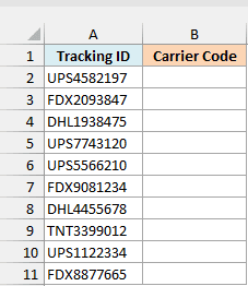
I want to pull just the carrier code out of every ID at once.
Here is the formula:
=LEFT(A2:A11,3)
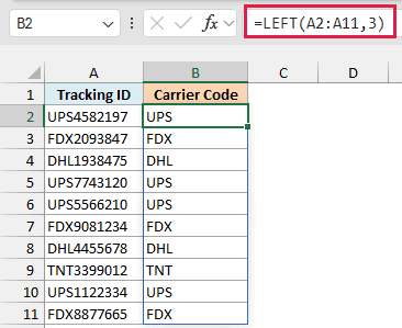
Because I handed LEFT the whole range A2:A11, the results spill down column B on their own. You type the formula once in B2 and Excel fills the rest.
The 3 tells LEFT to grab the first three characters of each string, so UPS4582197 becomes UPS and FDX2093847 becomes FDX.
Pro Tip: The spilling version needs Microsoft 365 or Excel 2021. On older versions, put =LEFT(A2,3) in B2 and copy it down the column.
Example 2: Extract Text Before a Delimiter Using LEFT and FIND
Now let’s handle strings where the part you want isn’t a fixed length. This is where LEFT teams up with the FIND function.
Below I have a list of full names in column A. I want just the first name from each one, but names are all different lengths, so a fixed number won’t work.
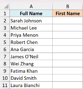
I want to pull everything before the first space in each name.
Here is the formula:
=LEFT(A2:A11,FIND(" ",A2:A11)-1)
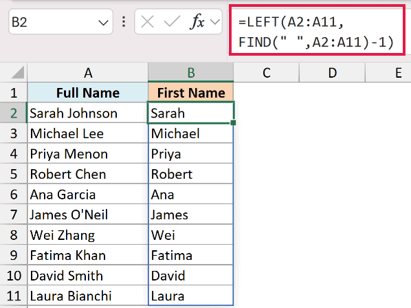
How this formula works:
- FIND(” “,A2:A11) locates the position of the first space in each name. For “Sarah Johnson” that’s position 6.
- Subtracting 1 gives the number of characters before that space, so 5 for “Sarah”.
- LEFT then grabs that many characters, returning “Sarah”.
Since the space position is different for every name, the character count adjusts for each row. That’s what lets one formula handle names of any length.
Follow along with the example file
LEFT Function Examples.xlsx
Example 3: Match a Delimiter in Any Case Using LEFT and SEARCH
Here’s a variation that trips people up. Sometimes the delimiter you’re splitting on shows up in different cases, and FIND won’t cope with that.
Below I have a list of product size codes in column A, like 10X4 and 6×9. The letter separating the two numbers is sometimes uppercase and sometimes lowercase.
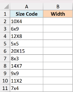
I want the first number (the width) from each code, whatever the case of the x.
Here is the formula:
=LEFT(A2:A11,SEARCH("x",A2:A11)-1)
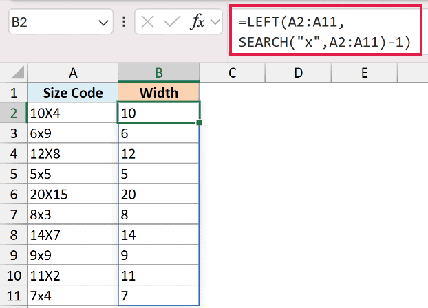
The key here is SEARCH instead of FIND. SEARCH ignores case, so it finds the x whether it’s written as X or x. It returns the position, we subtract 1, and LEFT grabs everything before it.
If you used FIND(“x”,…) here, it would fail on the uppercase codes like 10X4 and return a #VALUE! error, because FIND is case sensitive.
Example 4: Extract the Number and Make It Usable
This example covers the single biggest gotcha with LEFT: whatever it returns is always text, even when it looks like a number.
Below I have a list of prices in column A stored as strings, like 1200USD, where the amount is followed by a 3-letter currency code.
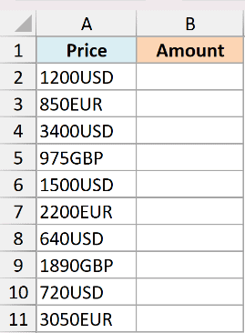
I want to separate the number from the code, and I want it as a real number I can add up.
First, let me pull the digits by chopping off the last 3 characters:
=LEFT(A2:A11,LEN(A2:A11)-3)
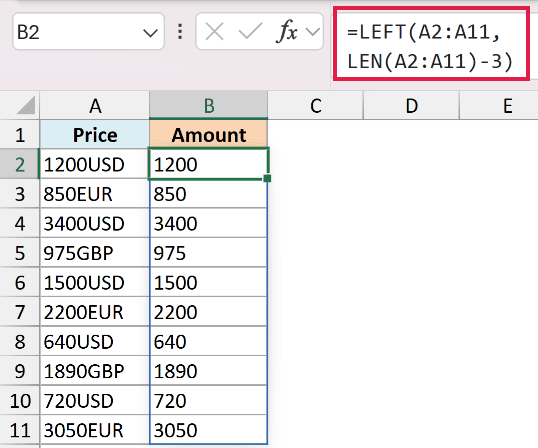
Here LEN counts the total characters in each string, and I subtract 3 for the currency code. LEFT then grabs everything up to it, so 1200USD becomes 1200.
But notice those results sit on the left side of the cell. That’s Excel’s way of telling you they’re text, not numbers. Try to SUM them and you’ll get 0.
To fix that, wrap the whole thing in the VALUE function:
=VALUE(LEFT(A2:A11,LEN(A2:A11)-3))
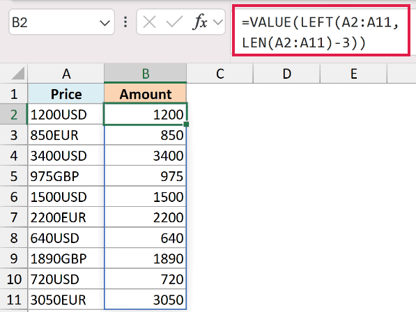
Now the results line up on the right, which means they’re real numbers. You can total them with a plain =SUM(), use them in calculations, or feed them into a chart.
Pro Tip: LEFT, RIGHT, and MID return text, but LEN and FIND return numbers. Arithmetic operators can convert numeric text automatically. Use VALUE when you want a numeric result, such as amounts to total with SUM.
Example 5: Categorize Rows by Their Prefix
LEFT is also handy inside a logical test, when the first few characters of a code tell you which group a row belongs to.
Below I have a list of invoice numbers in column A. Every one starts with either INT for international invoices or DOM for domestic ones.
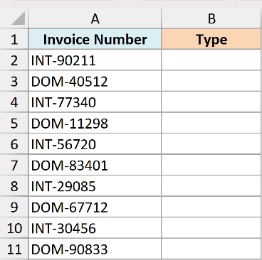
I want a label in column B that spells out the type based on that prefix.
Here is the formula:
=IF(LEFT(A2:A11,3)="INT","International","Domestic")
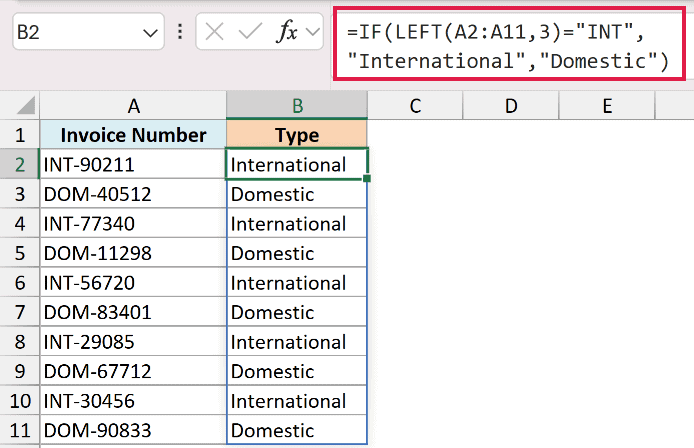
Here LEFT pulls the first 3 characters of each invoice number, and the IF function checks whether that equals “INT”. If it does, the row is labeled International, otherwise Domestic.
Because I passed the whole range in, the labels spill down the column automatically. This is a quick way to sort or filter records by a code prefix without a helper column of raw extracts.
LEFT vs RIGHT vs MID
LEFT is one of three text functions that pull a piece out of a string, and they’re often confused. Here’s the quick split.
- Use LEFT to grab characters from the start of a string.
- Use the RIGHT function to grab characters from the end, like the last 4 digits of a card number.
- Use the MID function to pull characters from the middle, starting at a position you choose.
They all share the same idea and often work together. In Excel 365 and Excel 2024, the TEXTBEFORE function can also grab text before a delimiter in one step, but LEFT paired with FIND still works everywhere and is worth knowing.
Tips & Common Mistakes
A few things to keep in mind when you use LEFT:
- LEFT always returns text. Even a result like “1200” is text, not a number. Arithmetic can convert it automatically, but SUM ignores text in cells. Wrap LEFT in VALUE to convert the result before totaling it with SUM.
- num_chars defaults to 1. If you forget the second argument, LEFT returns just the first character. Always spell out how many characters you want.
- FIND is case sensitive, SEARCH is not. When you split on a delimiter that might change case, use SEARCH so an uppercase letter doesn’t break the formula.
- Watch for extra spaces. A leading space throws off your character count. Run the text through the TRIM function first if the data is messy.
- num_chars can’t be negative. If a FIND lookup fails and returns an error, the whole LEFT formula errors out. Wrap it in IFERROR if some rows might not contain the delimiter.
Wrapping Up
LEFT is a small function you’ll reach for constantly once it clicks.
Start with a fixed number of characters, pair it with FIND or SEARCH when the length varies, and remember to wrap it in VALUE whenever you need a real number back.
I hope you found this tutorial helpful. If you get stuck on a LEFT scenario, it usually comes down to one of the common mistakes above.
Other Excel Articles You May Also Like:
