Separate Text and Numbers in Excel (4 Easy Ways)

Sometimes you may have the text and numeric data in the same cell, and you may have a need to separate the text portion and the number portion in different cells.

While there is no inbuilt method to do this specifically, there are some Excel features and formulas you can use to get this done.

In this tutorial, I will show you 4 simple and easy ways to separate text and numbers in Excel.

Let’s get to it!

Separate Text and Numbers Using Flash Fill

Below I have the employee data in column A, where the first few alphabets indicate the department of the employee and the numbers after it indicates the employee number.

From this data, I want to separate the text part and the number part and get these into two separate columns (columns B and C).

The first method that I want to show you to separate text and numbers in Excel is by using Flash Fill.

Flash Fill (introduced in Excel 2013) works by identifying patterns based on user input.

So if I manually enter the expected result in column B, Flash Fill will try and decipher the pattern and give me the result for all the cells in that column.

Below are the steps to separate the text part from the cell and get it in column B:

1. Select cell B2
2. Manually enter the expected result in cell B2, which would be MKT

3. With cell B2 selected, place the cursor at the bottom right part of the selection. You’ll notice that the cursor changes into a plus icon (this is called Fill Handle)

4.  Hold the left mouse/trackpad key and drag the Fill Handle to fill the cells. Don’t worry if the cells are filled with the same text
5. Click on the Auto Fill Options icon and then select the ‘Flash Fill’ option

The above steps would extract the text part from the cells in column A and give you the result in column B.

Note that in some cases, Flash Fill may not be able to identify the right pattern. In such cases, it would be best to enter the expected result in two or three cells, use the Fill Handle to fill the entire column, and then use Flash Fill on this data.

You can follow the same process to extract the numbers in column C. All you need to do is enter the expected result in cell C2 (step 2 in the process laid out above)

Note that the result you get from Flash Fill is static and would not update in case you change the original data in column A. If you want the result to be dynamic, you can use the formula method covered next.

Also read: Split Text into Multiple Rows in Excel

Separate Text and Numbers Using Formula

Below I have the employee data in column A and I want to use a formula to extract only the text part and put it in column B and extract the number part and put it in column C.

Since the data is not consistent (i.e., the alphabets in the department code and the numbers in the employee number are not of the consistent length), I cannot use the LEFT or RIGHT function to extract only the text portion or only the number portion.

Below is the formula that will extract only the text portion from the left:

=LEFT(A2,MIN(IFERROR(FIND({0,1,2,3,4,5,6,7,8,9},A2),""))-1)

And below is the formula that will extract all the numbers from the right:

=MID(A2,MIN(IFERROR(FIND({0,1,2,3,4,5,6,7,8,9},A2),"")),100)

How does this formula work?

Let me first explain the formula that we use to separate the text part on the left.

=LEFT(A2,MIN(IFERROR(FIND({0,1,2,3,4,5,6,7,8,9},A2),””))-1)

The FIND part in the formula finds the position of digits 0 to 9 in cell A2. In case it finds that digit in cell A2, it returns the position of that digit, and in case it is not able to find that digit, then it returns the value error (#VALUE!)

For cell A2, it gives a result as shown below:

{#VALUE!,4,#VALUE!,#VALUE!,#VALUE!,6,#VALUE!,5,#VALUE!,#VALUE!}

• For 0, it returns #VALUE! as it cannot find this digit in cell A2
• For 1, it returns 4 as that is the position of the first occurrence of 1 in cell A2
• and so on…

This FIND formula is then wrapped inside the IFERROR function, which removes all the value errors but leaves the numbers.

The result of it looks like as shown below:

{“”,4,””,””,””,6,””,5,””,””}

The MIN function then goes through the above result and gives us the minimum value from the results. Since each number in the array represents the position of that corresponding number, the minimum value tells us where the numerical value starts in the cell.

Now that we know where the numerical values start, I have used the LEFT function to extract everything before this position (which would be all the text in the cell).

Similarly, you can use the same formula with a minor tweak to extract all the numbers after the text. To extract the numbers, where we know the starting position of the first digit, use the MID function to extract everything starting from that position.

And what if the situation is reversed – where we have the numbers first and the text later and we want to separate the numbers and text?

You can still use the same logic with one minor change – instead of finding the minimum value that gives us the position of the 1st digit in the cell, you need to use the MAX function To find the position of the last digit in this cell. Once you have it, you can again use the LEFT function or the MID function to separate the numbers and text.

Separate Text and Numbers Using VBA (Custom Function)

While you can use the formulas shown above to separate the text and numbers in a cell and extract these into different cells – if this is something you need to do quite often, you also have the option to create your own custom function using VBA.

The benefit of creating your own function would be that it would be a lot easier to use (with just one function that takes only one argument).

You can also save this custom function VBA code into the Personal Macro Workbook so that it would be available in all your Excel workbooks.

Below the VBA code that could create a function ‘GetNumber’ that would take the cell reference as the input argument, extract all the numbers in the cell, and give it as the result.

'Code created by Sumit Bansal from https://trumpexcel.com
'This code will create a function that can separate numbers from a cell
Function GetNumber(CellRef As String)
Dim StringLength As Integer
StringLength = Len(CellRef)
For i = 1 To StringLength
If IsNumeric(Mid(CellRef, i, 1)) Then Result = Result & Mid(CellRef, i, 1)
Next i
GetNumber = Result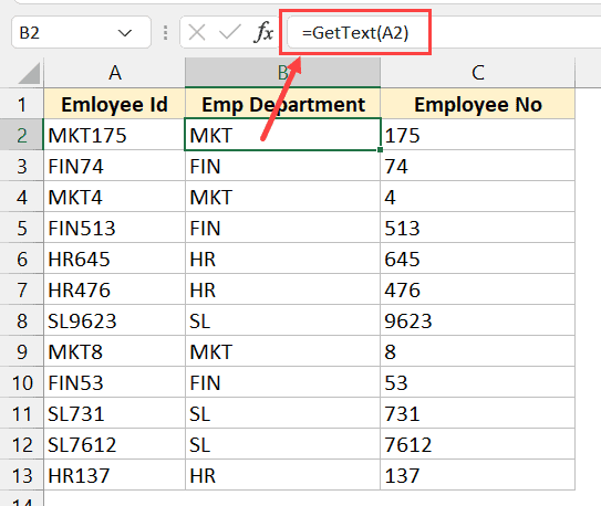
End Function

And below the VBA code that would create another function ‘GetText’ that would take the cell reference as the input argument and give you all the text from that cell

'Code created by Sumit Bansal from https://trumpexcel.com
''This code will create a function that can separate text from a cell
Function GetText(CellRef As String)
Dim StringLength As Integer
StringLength = Len(CellRef)
For i = 1 To StringLength
If Not (IsNumeric(Mid(CellRef, i, 1))) Then Result = Result & Mid(CellRef, i, 1)
Next i
GetText = Result
End Function

Below are the steps to add this code to your excel workbook so that this function becomes available for you to use in the worksheet:

1. Click the Developer tab in the ribbon
2. Click on the Visual Basic icon

3. In the Visual Basic editor that opens up, you would see the Project Explorer on the left. This would have the workbook and the worksheet names of your current Excel workbook. If you don’t see this, click on the View option in the menu and then click on Project Explorer

4. Select any of the sheet names (or any object) for the workbook in which you want to add this function
5. Click on the Insert option in the top toolbar and then click on Module. This will insert a new module for that workbook

6. Double click on the module icon in ‘Project Explorer’. This will open the module code window.

7. Copy and paste the above custom function code into the module code window

8. Close the VB Editor

With the above steps, we have added the custom function code to the Excel workbook.

Now you can use the functions =GETNUMBER or =GETTEXT just like any other worksheet function.

Note – Once you have the macro code in the module code window, you need to save the file as a Macro Enabled file (with the .xlsm extension instead of the .xlsx extension)

If you often have a need to separate text numbers from cells in Excel, it would be more efficient if you copy these VBA codes for creating these custom functions, and save these in your Personal Macro Workbook.

You can learn how to create and use Personal Macro Workbook in this tutorial I created earlier.

Once you have these functions in the Personal Macro Workbook, you would be able to use these on any Excel workbook on your system.

One important thing to remember when using functions that are stored in Personal Macro Workbook – you need to prefix the function name with =PERSONAL.XLSB!. For example, if I want to use the function GETNUMBER in a workbook in Excel, and I have saved the code for it in the postal macro workbook, I will have to use =PERSONAL.XLSB!GETNUMBER(A2)

Separate Text and Numbers Using Power Query

Power Query is slowly becoming my favorite feature in Excel.

If you’re already using Power Query as a part of your workflow, and you have a data set where you want to separate the text and numbers into separate columns, Power Query will do it in a few clicks.

When you have your data in Excel and you want to use Power Query to transform that data, one prerequisite is to convert that data into an Excel Table (or a named range).

Below I have an Excel Table that contains the data where I want to separate the text and number portions into separate columns.

Here are the steps to do this:

1. Select any cell in the Excel Table
2. Click the Data tab in the ribbon

3. In the Get and Transform group, click on the ‘From Table/Range’

4. In the Power Query editor that opens up, select the column from which you want to separate the numbers and text
5. Click the Transform tab in the Power Query ribbon

6. Click on the Split Column option

7. Click on ‘By Non Digit to Digit’ option.

8. You’ll see that the column has been split into two columns where one has only the text and the other only has the numbers

8. [Optional] Change the column names if you want
9. Click the Home tab and then click on Close and Load. This will insert a new sheet and give us the output as an Excel Table.

The above steps would take the data from the Excel Table we originally had, use Power Query to split the column and separate the text and the number parts into two separate columns, and then give us back the output in a new sheet in the same workbook.

Note that we used the option ‘By Non-Digit to Digit’ option in step 7, which means that every time there is a change from a non-digit character to a digit, a split would be made. If you have a dataset where the numbers are first followed by text, you can use the ‘By Digit to Non-Digit’ option

Now let me tell you the best part about this method. Your original Excel Table (which is the data source) is connected to the output Excel Table.

So if you make any changes in your original data, you don’t need to repeat the entire process. You can simply go to any cell in the output Excel Table, right click and then click on Refresh.

Power query would run in the back end, check the entire original data source, do all the transformations that we did in the steps above, and update your output result data.

This is where Power Query really shines. If there is a set of transformations that you often need to do on a data set, you can use Power Query to do that transformation once and set the process. Excel would create a connection between the original data source and the resulting output data and remember all the steps you had taken to transform this data.

Now, if you get a new data set you can simply put it in the place of your original data and refresh the query, and you will get the result in a few seconds. Alternatively, you can simply change the source in Power Query from the existing Excel table to some other Excel Table (in same or different workbook).

So these are four simple ways you can use to separate numbers and text in Excel. if this is a once-in-a-while activity, you’re better off using Flash Fill or the formula method.

And in case this is something you need to do quite often, then I would suggest you consider the VBA method where we created a custom function or the Power Query method.

I hope you found this Excel tutorial useful.

Other Excel tutorials you may also like:

• Separate First and Last Name in Excel (Split Names Using Formulas)
• How to Convert Numbers to Text in Excel
• Convert Text to Numbers in Excel – A Step By Step Tutorial
• How to Compare Text in Excel
• How to Quickly Combine Cells in Excel
• How to Combine First and Last Name in Excel
• How to Extract the First Word from a Text String in Excel (3 Easy Ways)
• Extract Numbers from a String in Excel (Using Formulas or VBA)
• How to Extract a Substring in Excel (Using TEXT Formulas)