

If you want to pull a few characters out of the middle of a text string, like a code buried inside an ID or a name sitting between two others, the MID function is what you need.
You tell it where to start and how many characters to grab, and it hands back exactly that piece.
In Excel 365, you can also feed MID a range and the results spill into the cells below, so one formula fills the whole column. In this article, I’ll show you how to use MID with a few practical examples.
Follow along with the example file
MID Function Examples.xlsx
MID Function Syntax
Here is the syntax of the MID function:
=MID(text, start_num, num_chars)
- text – The text string you want to pull characters from.
- start_num – The position of the first character you want, counting from 1.
- num_chars – How many characters to return, starting at that position.
All three arguments are required.
When to Use MID in Excel
Use the MID function when you need to:
- Pull a fixed set of characters from a set position in a code or ID.
- Extract text that sits between two markers (spaces, parentheses, hyphens) by pairing MID with FIND.
- Break a fixed-format string, like a text date or a SKU, into its separate parts.
- Grab a variable-length chunk of text by combining MID with LEN.
Let me show you how this works with a few practical examples.
Example 1: Extract Characters From the Middle (Fixed Position)
Let’s start with a simple example.
Below is a dataset of shipment codes in column A. Each code follows the same pattern, with a three-digit warehouse number sitting right after the “SH-” prefix.
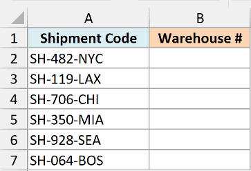
I want to pull out just that three-digit warehouse number from every code.
Here is the formula:
=MID(A2:A7,4,3)
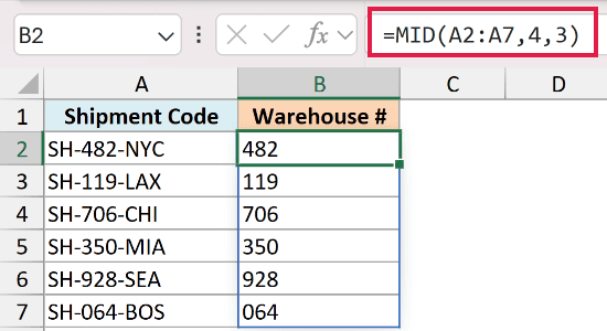
Here, MID starts at position 4 (the first digit after “SH-“) and grabs 3 characters. Since the number always sits in the same spot, the fixed start and length work for every row.
I fed MID the whole range A2:A7 in one go, so the result spills down the column automatically. In older versions of Excel, you would write =MID(A2,4,3) for the first row and drag it down.
Pro Tip: Position counting starts at 1, not 0. The first character of the string is position 1, so “SH-” occupies positions 1, 2, and 3.
Example 2: Extract the Middle Name From a Full Name
Here’s a more common scenario.
Below is a list of full names in column A. Each name has a first name, a middle name, and a last name, separated by spaces.
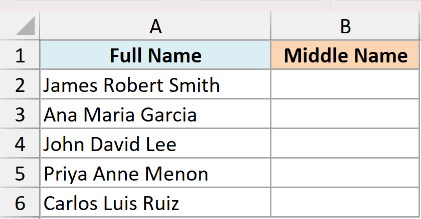
I want to pull out just the middle name from each one.
The middle name doesn’t start at a fixed spot, so I use FIND to locate the two spaces around it. Here is the formula:
=MID(A2,FIND(" ",A2)+1,FIND(" ",A2,FIND(" ",A2)+1)-FIND(" ",A2)-1)
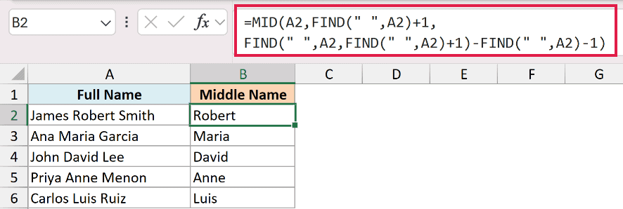
How this formula works:
FIND(" ",A2)finds the first space. Adding 1 gives MID the position right after it, where the middle name begins.FIND(" ",A2,FIND(" ",A2)+1)finds the second space by starting the search just past the first one.- Subtracting the first space position from the second (and one more for the space itself) gives the length of the middle name.
I kept this one per row so the nested FIND is easier to follow. In Excel 365 you can point it at the whole range with A2:A6 and let it spill.
Example 3: Extract Text Between Parentheses
Now let’s look at pulling text out from between two specific characters.
Below is a dataset of product names in column A. Each one has a SKU code tucked inside parentheses at the end.
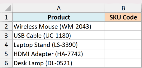
I want to extract just the SKU code from inside the parentheses.
Here is the formula:
=MID(A2,FIND("(",A2)+1,FIND(")",A2)-FIND("(",A2)-1)
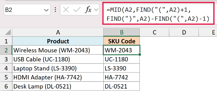
FIND locates the opening parenthesis, and adding 1 moves the start just inside it. For the length, MID takes the position of the closing parenthesis, subtracts the position of the opening one, and drops 1 so the brackets themselves are left out.
This same approach works for square brackets or any other pair of markers. Just swap the characters inside the FIND calls.
Example 4: Extract a Segment From an ID at Known Positions
Here’s a scenario you run into a lot with structured IDs.
Below is a list of student IDs in column A. Each ID packs three pieces into one string: the enrollment year, a three-letter subject code, and a roll number, all separated by hyphens.
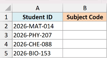
I want to pull out the three-letter subject code, which always sits at the same position.
Here is the formula:
=MID(A2:A5,6,3)
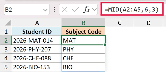
The subject code starts at position 6 (right after the four-digit year and its hyphen) and runs 3 characters. Because every ID follows the same layout, one spilling formula handles the whole column.
Pro Tip: MID isn’t only for the middle. Set start_num to 1 and it behaves like LEFT, so =MID(A2,1,4) would pull the “2026” year from the front of the same ID.
Example 5: Split a Text-Formatted Date Into Its Parts
Let’s use MID to break one string into separate pieces.
Below is a column of dates stored as text in the YYYYMMDD format (for example, 20260715). Excel reads these as plain text, not real dates.
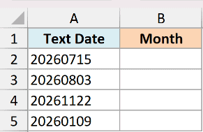
I want to pull out the two-digit month, which sits in the middle of each string.
Here is the formula:
=MID(A2:A5,5,2)
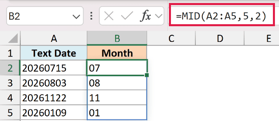
The month always occupies positions 5 and 6, so MID starts at 5 and grabs 2 characters.
To split out the rest, the year is positions 1 to 4 and the day is positions 7 to 8. You could also pull that trailing day with the RIGHT function.
Pro Tip: MID always returns text, even when the result looks like a number. If you need “07” as a real value for math, wrap the formula in VALUE, like =VALUE(MID(A2,5,2)).
Example 6: Use MID With LEN for a Dynamic Length
Let’s finish with a case where you don’t know how long the part you want is.
Below is a dataset of region labels in column A. Each one has a short prefix, a hyphen, and then a region name that varies in length from row to row.
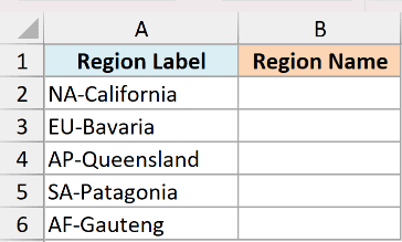
I want everything after the first hyphen, no matter how long the region name is.
Here is the formula:
=MID(A2,FIND("-",A2)+1,LEN(A2))
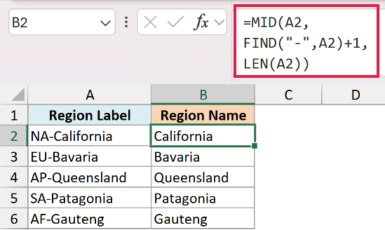
FIND locates the hyphen and MID starts just after it. For the length, I pass in LEN(A2), which is the length of the whole string.
That’s more characters than actually remain, but MID never overshoots. When you ask for more characters than are left, it simply returns everything through the end of the string.
Tips & Common Mistakes
- MID always returns text. Even when the extracted characters are all digits, the result is text. Wrap it in VALUE if you need a real number for calculations.
- Positions start at 1. The first character is position 1, not 0. Off-by-one start values are the most common MID mistake.
- A start_num past the end returns a blank. If start_num is greater than the length of the text, MID returns an empty string, not an error.
- Bad arguments trigger #VALUE!. If start_num is less than 1, or num_chars is negative, MID returns the #VALUE! error.
- num_chars can safely overshoot. Asking for more characters than remain just returns the rest of the string, which pairs nicely with LEN.
- FIND is case-sensitive. If you need case-insensitive matching (or wildcards) to locate your start position, use SEARCH in place of FIND.
MID is one of those functions that looks basic but does a lot of heavy lifting once you pair it with FIND and LEN.
Whether you’re pulling a code from an ID, a name from between two others, or a chunk of variable-length text, it comes down to telling MID where to start and how many characters to take.
Work through the six examples above and you’ll be able to reach for MID confidently the next time you need a slice from the middle of your data.
Other Excel Articles You May Also Like:
