

If you want to generate a random number in Excel, the RAND function is the quickest way to do it. It gives you a random decimal between 0 and 1 without needing any input.
One thing to know upfront: RAND is volatile, so it recalculates every time the sheet changes or you press F9.
It also doesn’t spill. It returns one value per cell, so when you need a whole grid of random numbers at once, its dynamic array cousin RANDARRAY is the one that spills them for you.
In this article, I’ll show you how to use RAND to create random decimals, whole numbers, values in a set range, and even shuffle a list.
RAND Syntax
Here is the syntax of the RAND function:
=RAND()
RAND takes no arguments. You just type the function with an empty pair of parentheses and it returns a random decimal that is greater than or equal to 0 and less than 1.
When to Use RAND
Use the RAND function when you need to:
- Generate a random decimal between 0 and 1
- Create random numbers inside a custom range (like 50 to 80)
- Build sample or test data quickly
- Shuffle a list into a random order
Let me show you a few practical examples of how RAND works.
Example 1: Generate a Random Number Between 0 and 1
Let’s start with the simplest use of the function.
You don’t need any data for this one. Just pick any empty cell on a blank worksheet.
I want a single random decimal that sits somewhere between 0 and 1.
Here is the formula:
=RAND()
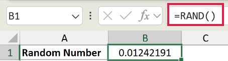
This returns a random decimal like 0.5824 or 0.1097. Every value is greater than or equal to 0 and less than 1, so you never get exactly 1.
Because RAND is volatile, the number changes every time the sheet recalculates. So the value you see in your screenshot will differ from mine.
Pro Tip: Press the F9 key to force a recalculation and watch the number change on demand.
Example 2: Generate a Random Number in a Range
Here’s a more useful scenario.
RAND on its own only gives you 0 to 1, but most of the time you want a number inside your own range. Again, no dataset is needed, so use any empty cell.
I want a random decimal between 50 and 80.
Here is the formula:
=RAND()*(80-50)+50
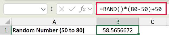
The pattern here is =RAND()*(b-a)+a, where a is the lowest value and b is the highest.
RAND gives a number from 0 to 1. Multiplying by 30 (which is 80 minus 50) stretches it to a 0-to-30 range, and adding 50 shifts it up so the result lands between 50 and 80.
Example 3: Generate a Random Whole Number
Now let’s get a whole number instead of a long decimal.
You can wrap RAND inside the INT function to chop off everything after the decimal point. No dataset is needed here either.
I want a random whole number between 1 and 100.
Here is the formula:
=INT(RAND()*100)+1
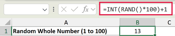
Here is how this formula works:
RAND()*100gives a decimal from 0 up to (but not including) 100.INT(...)drops the decimal part, leaving a whole number from 0 to 99.+1shifts the result so it lands between 1 and 100.
Pro Tip: If you only need random whole numbers, the RANDBETWEEN function does this in one step with =RANDBETWEEN(1,100).
Example 4: Random Decimal With Set Precision
Sometimes you want a random decimal, but not one that runs to 15 digits.
You can round the result to as many decimal places as you like by wrapping the formula in the ROUND function. No dataset is needed.
I want a random rating between 1 and 5, rounded to 2 decimal places.
Here is the formula:
=ROUND(RAND()*(5-1)+1,2)
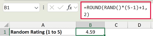
The inside part, RAND()*(5-1)+1, is the same range trick from Example 2, giving a decimal between 1 and 5.
The ROUND function then trims it to 2 decimal places, so you get clean values like 3.47 or 4.92 instead of a long string of digits.
Example 5: Shuffle a List in Random Order
Let’s use RAND to randomize a list.
Below is a small dataset with a list of employee names in column A. I want to randomize this list so the names end up in a random sequence.
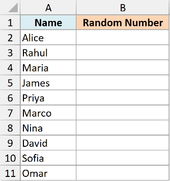
The classic way is to add a helper column of random numbers next to the list, then sort by it.
In cell B2, next to the first name, enter this formula and copy it down beside every name.
Here is the formula:
=RAND()
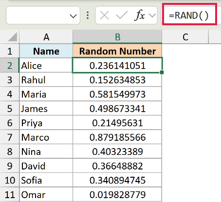
Now select any cell in the helper column and sort it (Data tab, Sort A to Z). Because the random numbers have no pattern, the names get shuffled into a random order.
If you have Excel 365 or 2021, there is a cleaner one-formula way that skips the helper column entirely.
Here is the formula:
=SORTBY(A2:A11,RANDARRAY(ROWS(A2:A11)))
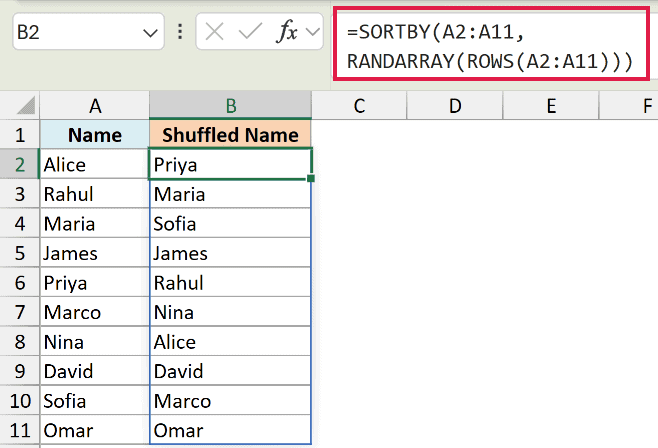
Here, RANDARRAY builds a list of random numbers with one value per name, and SORTBY uses those random values to reorder the names. The shuffled list spills into the cells below.
Pro Tip: To pick a single random winner instead of shuffling everyone, wrap it in INDEX: =INDEX(A2:A11,INT(RAND()*10)+1).
Example 6: Freeze Random Numbers So They Stop Changing
There is one catch with everything above. Since RAND is volatile, your numbers keep changing every time the sheet recalculates.
Below is a column of random numbers created with =RAND(). I want to lock these values so they stay put and stop refreshing.
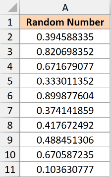
To freeze them, select the range of random numbers and copy it with Control + C. Then right-click the same selection and choose Paste Special, followed by Values.
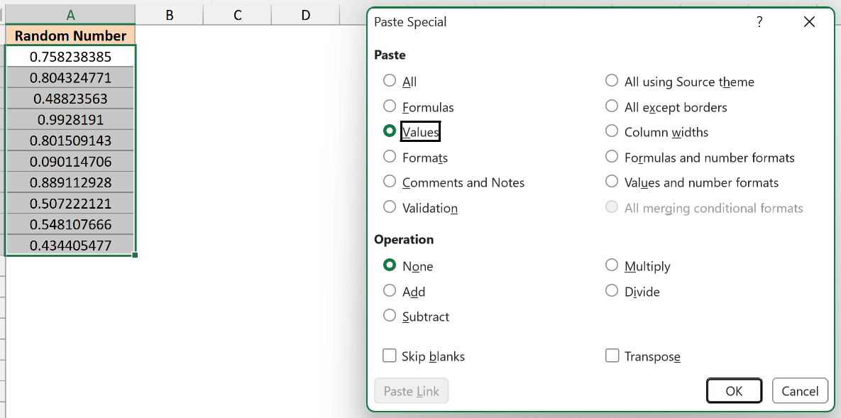
This replaces the live formulas with their current results as plain numbers. They will never change again, because there is no RAND formula left to recalculate.
Pro Tip: For a single cell, type =RAND() in the formula bar and press F9 before hitting Enter. Excel converts the formula to a static number on the spot.
Tips & Common Mistakes
- RAND is volatile. It recalculates on every edit, on every open, and whenever you press F9. This is why your saved values look different each time, and why screenshots of RAND never match.
- Freeze the values when you need them fixed. Copy the cells and use Paste Special, then Values, to convert the formulas into static numbers so they stop changing.
- RAND does not spill. It returns one value per cell. For a whole block of random numbers in a single formula, use RANDARRAY, which lets you set the rows, columns, and min and max in one shot.
- Don’t confuse the three random functions. RAND gives a decimal from 0 to 1, RANDBETWEEN gives a whole number between two values, and RANDARRAY spills an array of random numbers across a range.
That covers the main ways to use the RAND function in Excel. You’ve seen how to create random decimals, whole numbers, and values in a custom range, plus how to shuffle a list and freeze the results.
Once you’re comfortable with RAND, RANDBETWEEN and RANDARRAY are natural next steps for more control over your random numbers.
Other Excel Articles You May Also Like: