

The VALUETOTEXT function in Excel converts values to text, including numbers, TRUE or FALSE, and error values such as #N/A. You can also use it with cells that already contain text.
The result can look exactly like the original value, even though Excel now treats it as text. Dates and formatted numbers need a little more care because VALUETOTEXT doesn’t keep their original formatting.
In this tutorial, I’ll show you how to convert a column of values, use quotation marks to identify original text, and see what happens to formatted values and errors.
Follow along with the example file
VALUETOTEXT Function Examples.xlsx
VALUETOTEXT Function Syntax
Here is the syntax of the VALUETOTEXT function:
=VALUETOTEXT(value, [format])
- value is the value you want to convert to text. You can supply a value directly or refer to a cell or range of cells.
- format is optional. Use 0 for concise text or 1 for strict text.
If you leave out the format argument, Excel uses 0. This produces text without adding quotation marks around values that were already text.
With format set to 1, original text values get quotation marks around them. Numbers, logical values, and errors don’t get those surrounding quotes, although their results are still text.
The VALUETOTEXT function is available in Microsoft 365, Excel 2024, and Excel 2021 for Windows and Mac.
When to Use the VALUETOTEXT Function
Use this function when you need to:
- Convert numbers to text without applying a particular display format.
- Show which values in a mixed list were originally text.
- Record error labels as text while keeping the original cells available to inspect.
Let me show you how each of these works.
Example 1: Convert a Column of Numbers to Text
Let’s start with a column of ordinary numbers.
Below I have a list of club supplies and their quantities, and I want to convert the quantities to text in column C.
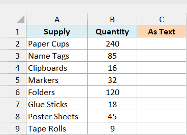
Enter the following formula in cell C2 and press Enter:
=VALUETOTEXT(B2:B9)
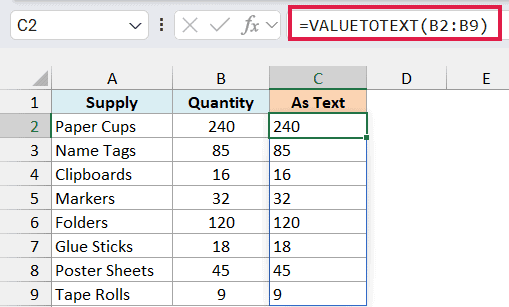
The formula converts all eight quantities at once. Its results spill into C2:C9 automatically, so you don’t need to copy the formula down.
The 240 for Paper Cups still looks like 240, but the result is now text. The original quantity in column B remains a number.
You can confirm the change with the ISTEXT function, which returns TRUE when a value is text. Enter this formula in cell D2:
=ISTEXT(C2:C9)
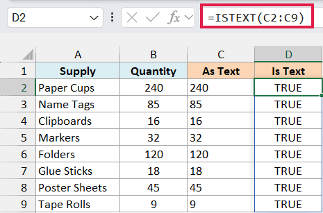
Every result is TRUE, confirming that all eight converted quantities are text. Keep the original numbers in column B for calculations that need numeric inputs.
Example 2: Use Strict Format to Identify Text
Now let’s look at values that can be hard to tell apart just by looking at them.
Below I have a list of package label fields, and I want to show which recorded values were originally text in column C.
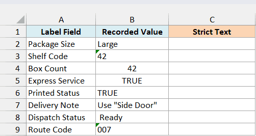
Enter the following formula in cell C2:
=VALUETOTEXT(B2:B9,1)
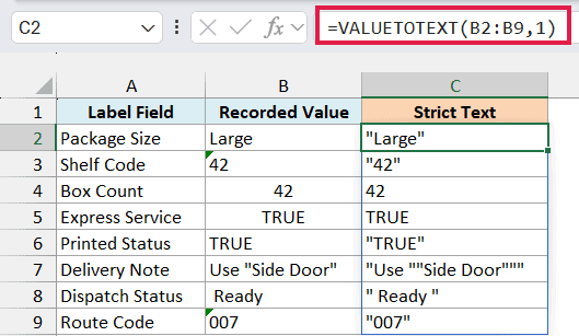
The second argument is 1, so this formula uses strict format. It adds quotation marks around each value that was already text.
For example, the Shelf Code is stored as text, so its result is "42". The Box Count is the number 42, so its result has no surrounding quotes.
The same distinction applies to TRUE. Express Service contains the logical value TRUE and returns TRUE, while Printed Status contains the word TRUE as text and returns "TRUE".
Those quotes are actual characters in the result. They tell you about the original value; both the quoted and unquoted outputs in column C are text.
The Delivery Note also shows how strict format handles quotation marks that are already inside text. Use "Side Door" becomes "Use ""Side Door""", with the inner quotation marks doubled.
The spaces around Ready remain inside its surrounding quotes, and the text code 007 keeps its leading zeros. Strict format exposes these details without changing the source cells.
Example 3: See What Happens to Number Formats
Converting a value to text doesn’t necessarily preserve what you see in the original cell.
Below I have booking details with date, currency, percentage, and custom number formats, and I want to see their text conversions in column C.
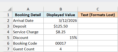
Enter the following formula in cell C2:
=VALUETOTEXT(B2:B7)
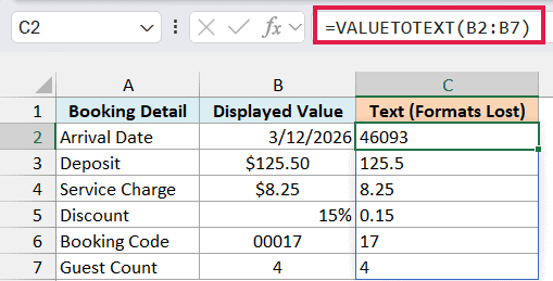
The arrival date displays as 3/12/2026, but the formula returns 46093. Excel stores dates as numbers, and 46093 is the underlying date value in this workbook.
The deposit displays as $125.50 and becomes 125.5. The discount displays as 15% and becomes 0.15, because that is the number stored in the percentage cell.
The booking code is the number 17 displayed with a custom format that adds leading zeros. VALUETOTEXT returns 17, so the zeros you see in 00017 are lost.
This differs from the text code 007 in the previous example. Its zeros are part of the text itself, so they remain in the result.
Important: VALUETOTEXT doesn’t preserve date, currency, percentage, or custom number formatting. When your text result needs a specific appearance, use the TEXT function with the format you want.
Example 4: Convert Excel Errors to Text
An error label can look the same before and after conversion, too.
Below I have order totals that include error values, and I want to convert all the entries to text in column C.
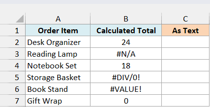
Enter the following formula in cell C2:
=VALUETOTEXT(B2:B7)
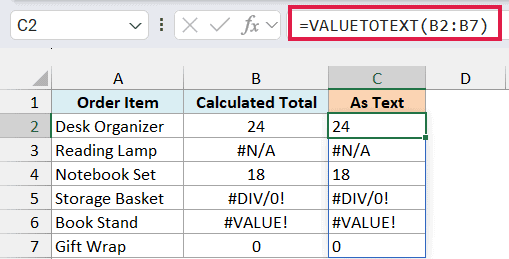
The numbers become text, just as they did in the first example. The #N/A, #DIV/0!, and #VALUE! errors become text containing those same labels.
Since the output still looks like an error, let’s check its type. Enter the following formula in cell D2:
=ISTEXT(C2:C7)
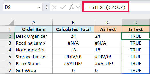
Every result is TRUE, including the rows showing #N/A, #DIV/0!, and #VALUE!. Those entries in column C are ordinary text strings, so they can be kept as a text record of the errors.
This conversion doesn’t fix the underlying problem. The original errors remain in column B, where you can investigate what caused them.
Use VALUETOTEXT when you need the underlying values as text. If the appearance of a date or formatted number matters, choose the formatting deliberately instead of relying on the source cell’s display.
Other Excel Articles You May Also Like:
