

The SERIESSUM function returns the sum of a power series. That’s a list of terms like 4 + 1.5x + 0.25x², where each term is a coefficient multiplied by x raised to a higher power.
You give it x, the starting power, the step between powers, and a range holding the coefficients. It’s handy for polynomials, trendline equations, and approximating functions like sine.
In this article, I’ll show you five examples, from a simple polynomial to a sine approximation you can check against the built-in SIN function.
Follow along with the example file
SERIESSUM Function Examples.xlsx
SERIESSUM Function Syntax
Here is the syntax of the SERIESSUM function:
=SERIESSUM(x, n, m, coefficients)
- x – The number you plug into the series. It has to be a single value, not a range.
- n – The power you raise x to in the first term.
- m – The amount the power goes up by for each following term.
- coefficients – The numbers that multiply each power of x, usually a range of cells.
SERIESSUM adds a1 × x^n + a2 × x^(n+m) + a3 × x^(n+2m) and so on, where a1, a2, a3 are the coefficients in the order they appear.
The number of values in coefficients decides how many terms you get. Three coefficients mean three terms.
Both n and m can be negative, and Example 5 uses a negative m.
The SERIESSUM function works in Excel for Microsoft 365, Excel 2024, 2021, 2019, and 2016, on both Windows and Mac.
When to Use the SERIESSUM Function
Use the SERIESSUM function when you need to:
- Calculate a polynomial whose coefficients are stored in cells
- Predict a value from a polynomial trendline equation
- Add terms that follow a power pattern, such as x, x³, x⁵
- Approximate a function like sine or cosine with a power series
- Add or remove terms by changing the coefficient range, without rewriting the formula
Let me show you five examples of how to use the SERIESSUM function.
Example 1: Calculate a Polynomial With SERIESSUM
Let’s start with a simple polynomial.
Below I have a parcel delivery fee made up of a base fee, a fee per kg, and a fee per kg squared, and I want to get the fee for the parcel weight in E1 in cell E2.
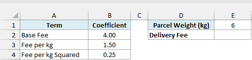
Here is the formula:
=SERIESSUM(E1,0,1,B2:B4)
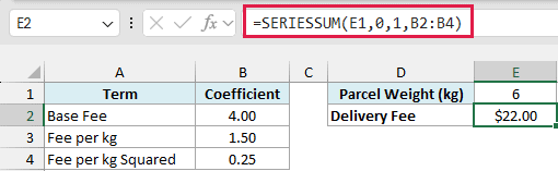
This returns $22.00 for a 6 kg parcel.
In this formula, E1 is the weight (x), 0 means the first term uses x to the power of 0, and 1 means the power goes up by 1 with each term. B2:B4 holds three coefficients, so Excel builds three terms.
That works out to 4 × 6^0 + 1.5 × 6^1 + 0.25 × 6^2, which is 4 + 9 + 9 = 22.
The squared term makes the fee climb faster as parcels get heavier. Doubling the weight from 6 kg to 12 kg takes the fee from $22.00 to $58.00, which is more than double.
Make sure the coefficient range starts below the header. If it includes the word Coefficient, SERIESSUM returns the #VALUE! error, because it can’t use text.
Important: Enter 0 for a term you don’t need, and never leave its cell blank. SERIESSUM skips a blank cell, so every coefficient after it slides down one power and the result is wrong.
Example 2: Calculate a Whole List in One Formula
Now let’s get the fee for a whole list of weights instead of just one.
Below I have a list of parcel weights in column A and the same fee coefficients in E2:E4, and I want to get the delivery fee for each weight in column B.
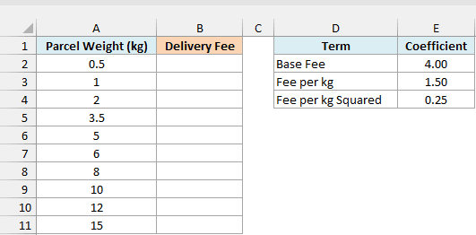
Here is the formula:
=MAP(A2:A11,LAMBDA(w,SERIESSUM(w,0,1,E2:E4)))
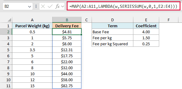
You can’t give SERIESSUM the whole range A2:A11 as x. It needs a single number, so a range returns the #VALUE! error.
The MAP function fixes that. It takes each weight in A2:A11 one at a time, passes it to the LAMBDA function as w, and SERIESSUM calculates the fee for it, with the results spilling down column B.
MAP and LAMBDA work in Excel 365 and Excel 2024. If you are using Excel 2021 or earlier, enter the below formula in cell B2 and then copy it down the range:
=SERIESSUM(A2,0,1,$E$2:$E$4)
The dollar signs lock the coefficient range, so it doesn’t move as you copy the formula down.
A weight of 0 would return the #NUM! error here, because the first term becomes 0 raised to the power of 0. That’s why the list starts at 0.5 kg.
Example 3: Start the Series at a Higher Power
Next, let’s look at what the n argument does.
Below I have the average spend per customer for each wave of a referral program, and the number of friends each customer invites in E1. I want to get the total revenue in cell E2.
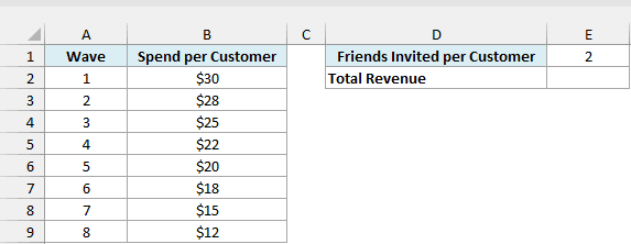
Here is the formula:
=SERIESSUM(E1,1,1,B2:B9)
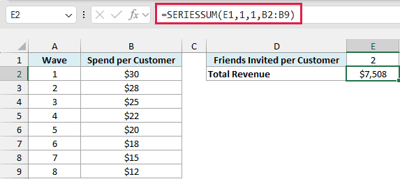
This returns $7,508.
The program starts with one customer, each customer invites 2 friends (the value in E1, which is our x), and I’m assuming every friend joins.
So wave 1 has 2 customers, wave 2 has 4, wave 3 has 8, and wave 8 has 256.
That’s 2 raised to the power of the wave number, which is why n is 1 and m is 1.
Each coefficient is the spend per customer for that wave. Wave 8 adds 256 × $12 = $3,072, even though its customers spend less than wave 1, because there are so many more of them.
If I had left n at 0, the first term would be 30 × 2^0 = 30, as if wave 1 had only one customer. The whole total would drop to $3,754.
Example 4: Approximate Sine With a Power Series
Now let’s put the m argument to work.
The sine of an angle can be approximated with a power series: x – x³/3! + x⁵/5! – x⁷/7! and so on. The powers go 1, 3, 5, 7, so n is 1 and m is 2.
The ! means factorial, so 3! is 3 × 2 × 1 = 6, and 5! is 120.
Below I have the term numbers 0 to 4 in column A and a list of angles in column D. I want to build the coefficients in column B first, then get the sine of each angle in column E.
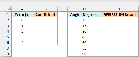
Here is the formula for the coefficients:
=(-1)^A2:A6/FACT(2*A2:A6+1)
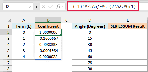
The (-1)^A2:A6 part flips the sign from one term to the next. The FACT function gives the factorial of 1, 3, 5, 7, and 9.
So the coefficients are 1, -1/3!, 1/5!, -1/7!, and 1/9!. Now here is the SERIESSUM formula that uses them:
=MAP(D2:D8,LAMBDA(a,SERIESSUM(RADIANS(a),1,2,B2:B6)))
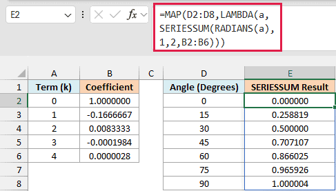
The series expects radians, so the RADIANS function converts each angle first. MAP passes the angles in one at a time, for the same reason as in Example 2.
With n as 1 and m as 2, the powers are 1, 3, 5, 7, and 9. B2:B6 holds five coefficients, so you get five terms.
To check the answers, here is the built-in SIN function in column F:
=SIN(RADIANS(D2:D8))
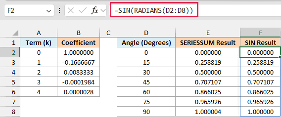
The two columns match to six decimals, except at 90 degrees.
There SERIESSUM gives 1.000004 instead of 1, because the series stops after five terms. More coefficients close that gap.
Excel 2021 can spill formulas but doesn’t have MAP and LAMBDA. So Excel 2021 needs a fallback only for the SERIESSUM results, and Excel 2019 or earlier needs all three.
If you are using Excel 2019 or earlier, enter the below formula in cell B2 and then copy it down to B6 to get the coefficients:
=(-1)^A2/FACT(2*A2+1)
If you are using Excel 2021 or earlier, enter the below formula in cell E2 and then copy it down to E8 to get the SERIESSUM results:
=SERIESSUM(RADIANS(D2),1,2,$B$2:$B$6)
And if you are using Excel 2019 or earlier, enter the below formula in cell F2 and copy it down to F8 for the SIN check:
=SIN(RADIANS(D2))
Pro Tip: You can approximate cosine the same way, with n at 0, m at 2, and the coefficients =(-1)^A2:A6/FACT(2*A2:A6). Just skip an angle of 0, which returns #NUM! when n is 0.
Example 5: Use Polynomial Trendline Coefficients Directly
This last example is for anyone who has added a polynomial trendline to a chart.
When you show the equation on a polynomial trendline, Excel lists the highest power first, like y = -2x² + 90x – 300. SERIESSUM normally starts from the lowest power, so it looks like you’d have to reverse the coefficients.
Below I have the coefficients of a trendline equation that predicts revenue from the ticket price, copied in the order the chart shows them. I want to get the predicted revenue for the price in E1 in cell E2.
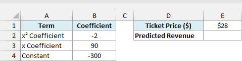
Here is the formula:
=SERIESSUM(E1,2,-1,B2:B4)
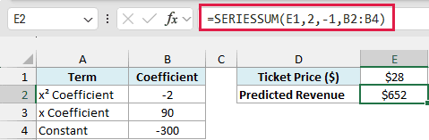
This returns $652 for a ticket price of $28.
The trick is the negative m. The first term uses the highest power, so n is 2, and m is -1.
That makes the powers go 2, 1, 0, which matches the order of the coefficients, so there’s nothing to reverse.
For a price of $28, the formula calculates -2 × 28^2 + 90 × 28 – 300, which is $652. For a third-order trendline, you’d start n at 3 and keep m at -1.
So that’s how the SERIESSUM function works. Use n for the starting power, m for the step, and the size of the coefficient range to decide how many terms you get.
I hope you found this Excel tutorial useful.
Other Excel Articles You May Also Like:
