How to Create a Waterfall Chart in Excel

A waterfall chart shows how a starting number goes up and down, one step at a time, until it reaches an ending number. A regular column chart won’t do it justice, because it shows each value as a separate bar with no running total.

In this article, I’ll show you how to create a waterfall chart with Excel’s built-in chart type and how to add subtotals to it. I’ll also show you how to build one with a stacked column chart in older versions of Excel.

What a Waterfall Chart Is Good For

A waterfall chart is great whenever you want to explain how you got from one number to another. Think of a profit bridge, a cash flow summary, or inventory changes over a period.

Each change bar starts where the previous bar ended and goes up or down by that amount. Increases push the total up, decreases pull it down, and totals sit flat on the baseline so you can read the start and end at a glance.

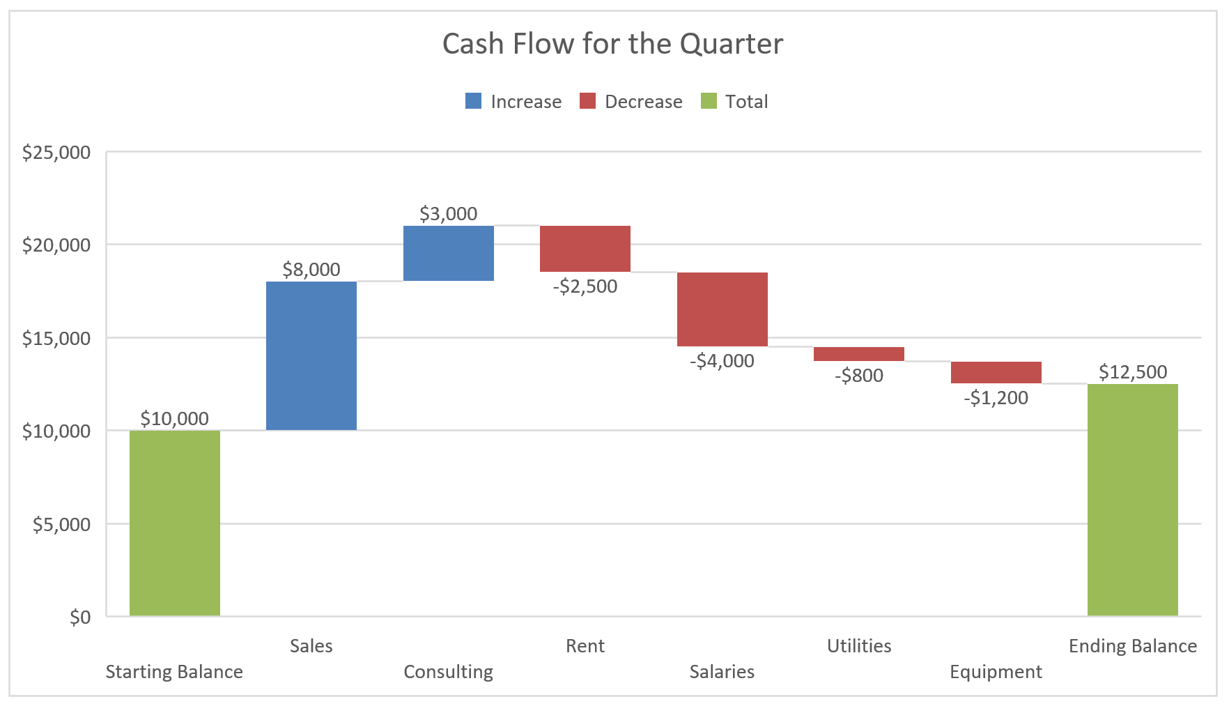
Below is the waterfall chart we’ll build in the first method, from a cash flow summary for one quarter.

Method 1: Create a Waterfall Chart Using the Built-In Chart Type (Recommended)

Let’s start with the easiest approach. Excel has a built-in Waterfall chart type, so you don’t need any helper columns or formulas.

The built-in Waterfall chart works in Excel 2016 and later, including Microsoft 365 and Excel for Mac. If you’re on Excel 2013 or older, use the stacked column method later in this article.

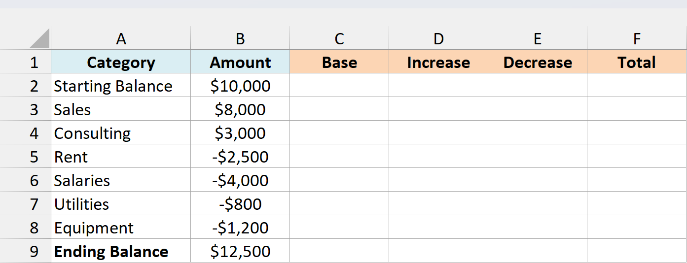
Below is a cash flow summary with the starting balance, the money that came in and went out during the quarter, and the ending balance, and I want to show how the starting balance turns into the ending one.

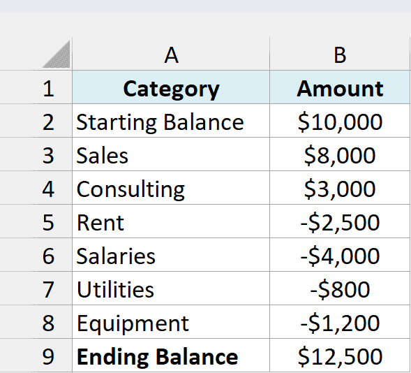
Anything that reduces the balance, like Rent or Salaries, is entered as a negative number in the Amount column. The chart uses the sign of each value to decide whether its bar goes up or down.

The Ending Balance in B9 is the formula =SUM(B2:B8), so it updates when you change any of the amounts above it.

Here are the steps to create a waterfall chart from this data:

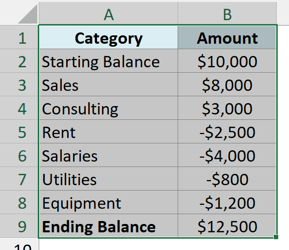
1. Select the data in A1:B9, including the headers.

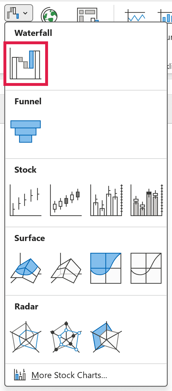
2. Click the Insert tab, click the Insert Waterfall, Funnel, Stock, Surface, or Radar Chart icon in the Charts group, and then click Waterfall.

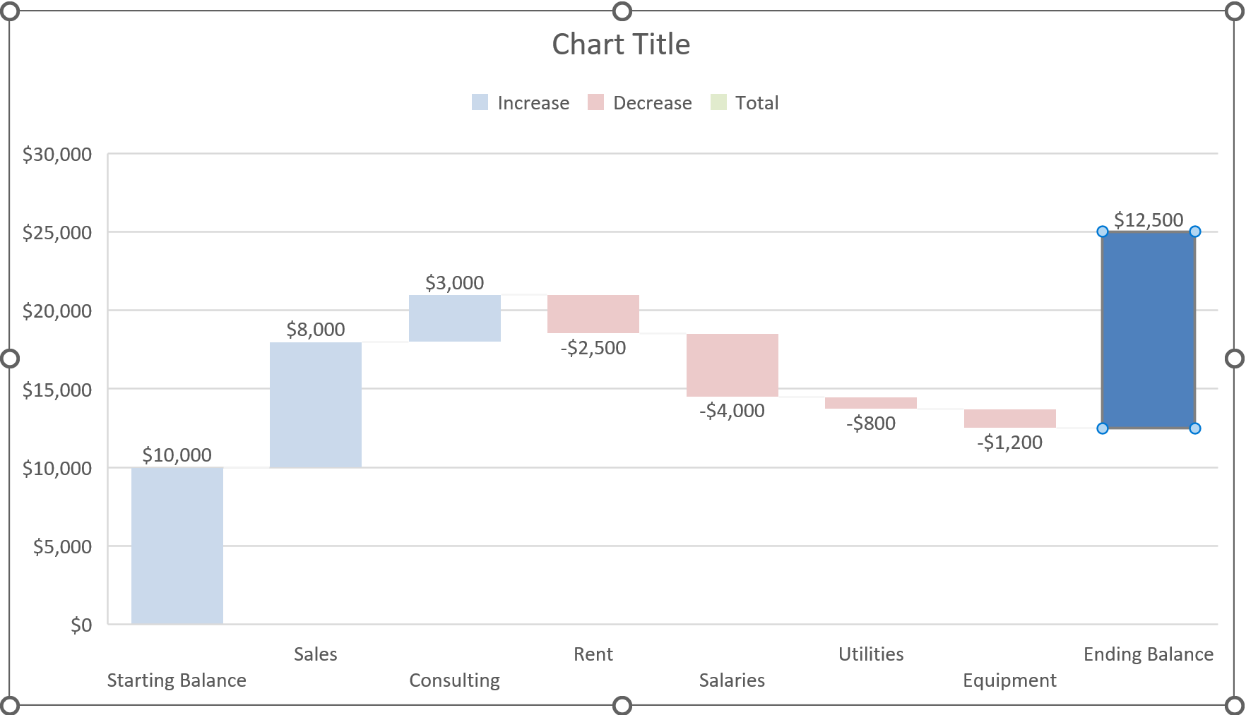
Excel drops a waterfall chart onto your sheet. The increases and decreases already look right, but the Ending Balance bar floats in mid-air instead of sitting on the baseline.

That’s because Excel treats every bar as a change by default, so it stacks the ending balance on top of everything before it.

The Starting Balance bar happens to start at zero anyway, but Excel still colors it as an increase. So you need to tell Excel that both of these bars are totals.

3. Click the Ending Balance bar once to select all the bars, and then click it again so only that one bar stays selected.

4. Right-click the selected bar and click Set as Total.

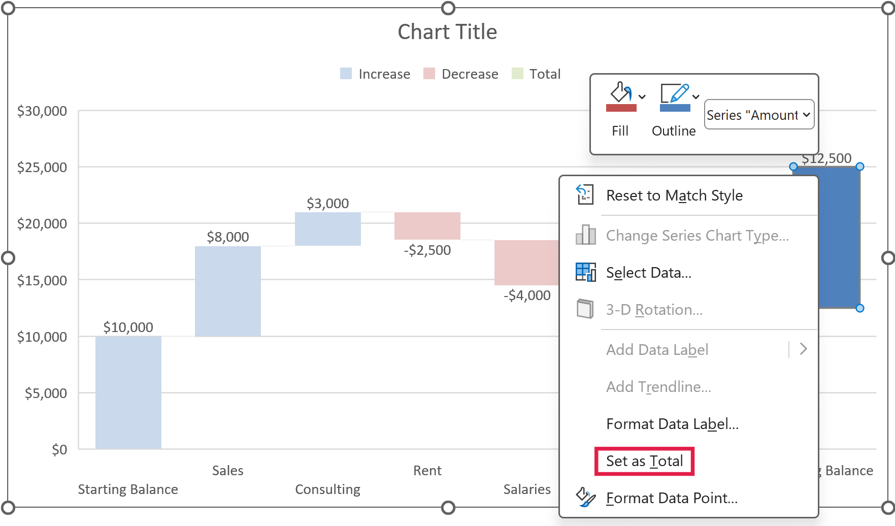
If you don’t see Set as Total in the menu (it shows Format Data Series instead of Format Data Point), the whole series is still selected. Click the bar once more so only that bar is selected, and then right-click it again.

5. Do the same for the Starting Balance bar. Click it twice so only that bar is selected, right-click it, and click Set as Total.

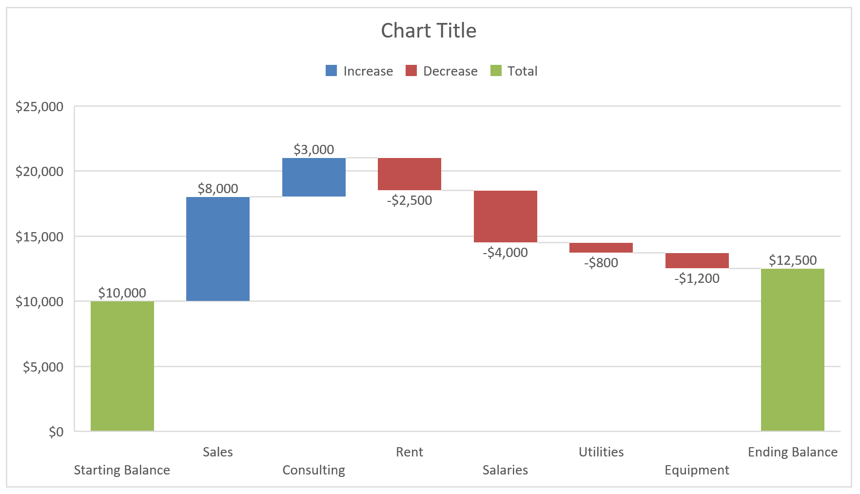
The Ending Balance now drops down to the baseline where it belongs. Both balance bars also pick up the Total color, so they read as totals and not as changes.

You can also right-click a single selected bar, click Format Data Point, and check the Set as total box in the pane. Unchecking that box turns the bar back into a change.

6. Click the Chart Title box, select the placeholder text, and type a title, such as Cash Flow for the Quarter.

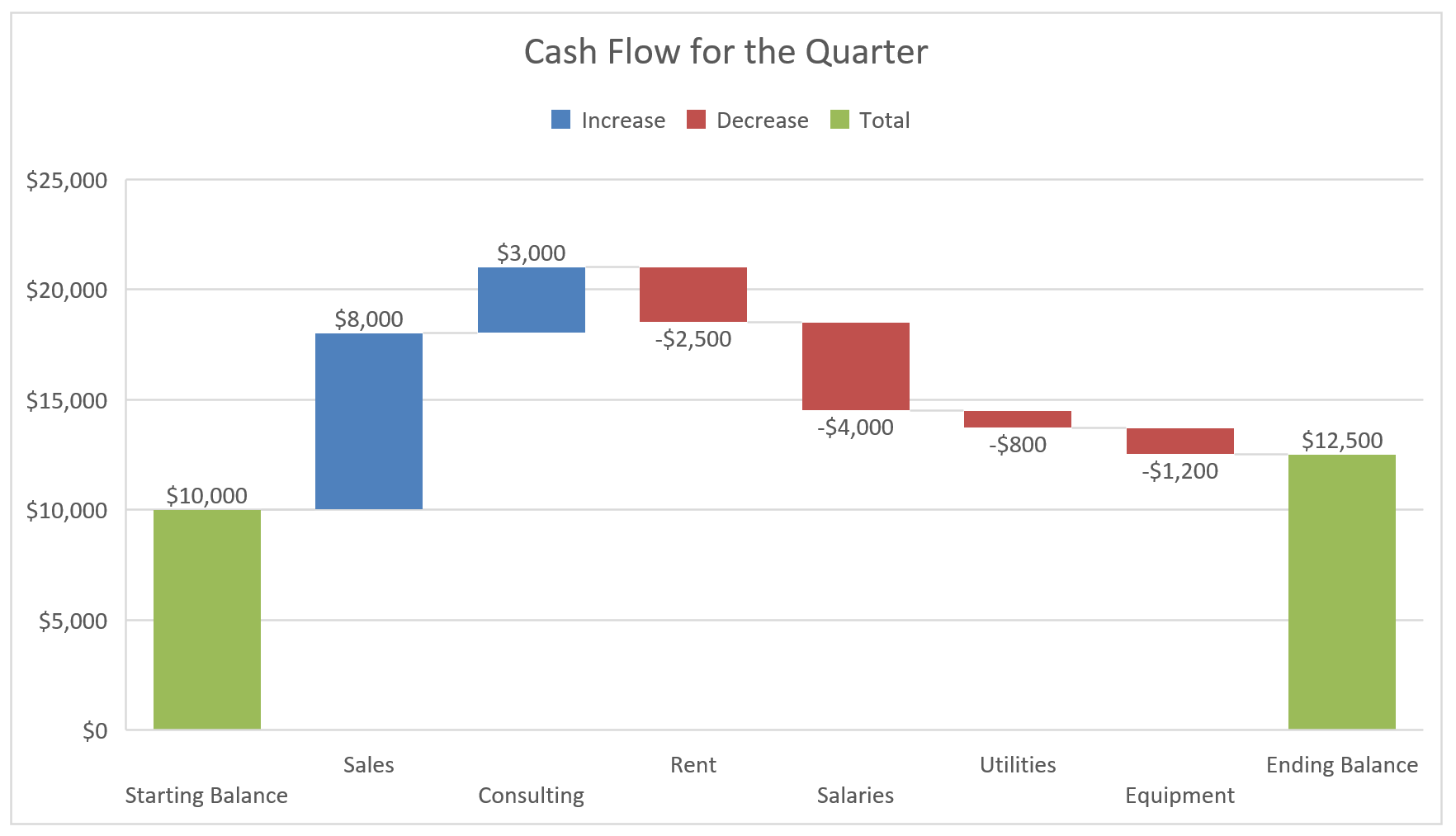
The built-in chart adds data labels on its own, so every bar already shows its amount.

The thin lines that join one bar to the next are called connector lines, and they’re on by default. For a cleaner look, click any bar once so all the bars are selected, right-click it, click Format Data Series, and uncheck Show connector lines.

Changing the Colors of the Bars

Excel uses three colors in a waterfall chart, one for increases, one for decreases, and one for totals. You can see which is which in the legend at the top of the chart.

A waterfall chart has only one data series. Increase, Decrease, and Total are groups of data points inside it, which is why you work through the legend to recolor them.

Here are the steps to change any of these colors:

1. Click the legend once to select it, and then click the Increase entry so only that entry is selected.

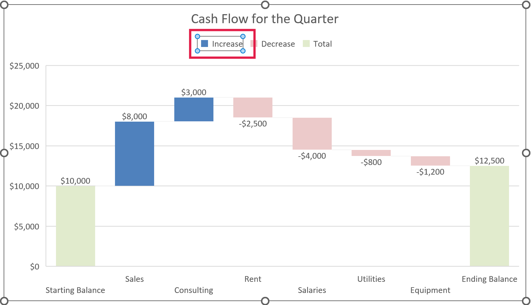
2. Right-click the Increase entry, click the Fill drop-down, and pick the color you want.

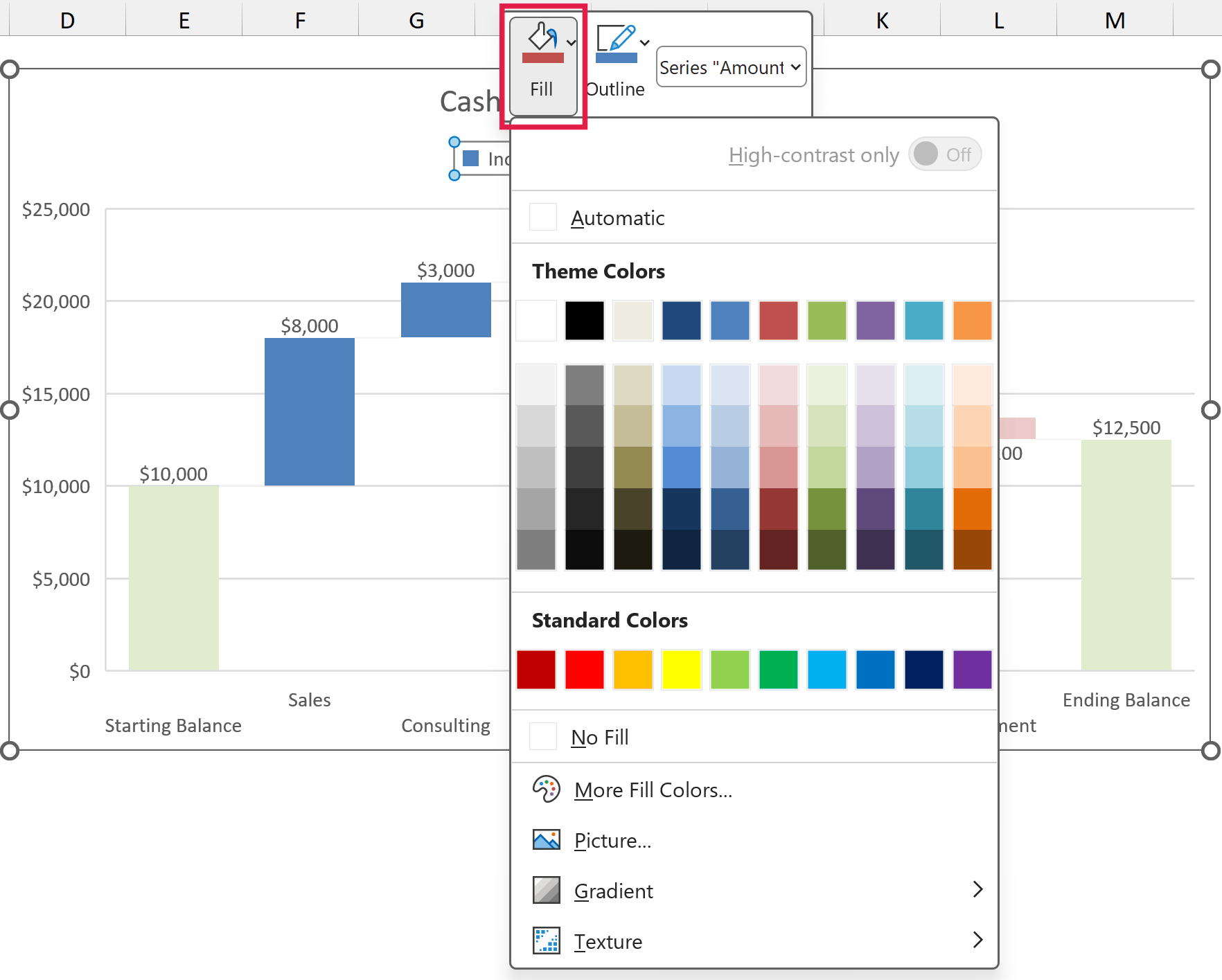
The color you pick applies to every increase bar in the chart. Repeat the same for the Decrease and Total entries.

A common choice is green for increases, red for decreases, and a neutral gray for totals.

The Increase, Decrease, and Total entries come from Excel, not from your data (the series itself is named Amount), so renaming the series won’t change them. If you need different wording, delete the legend and add your own text boxes instead.

Adding Subtotals to a Waterfall Chart

A waterfall chart doesn’t have to show totals only at the start and end. In a profit bridge, you’ll often want a subtotal partway through, like gross profit before the operating costs.

Below is a monthly profit breakdown with sales, returns, product costs, a Gross Profit row, the operating costs, and the Net Profit, and I want both profit rows to show up as totals in the chart.

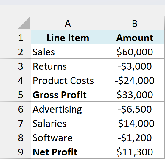
The key thing is that a subtotal row holds the running total, not a change. Gross Profit in B5 is =SUM(B2:B4), and Net Profit in B9 is =B5+SUM(B6:B8).

Net Profit can’t simply be =SUM(B2:B8), because that range includes the Gross Profit row, so the first three rows would get counted twice.

Here are the steps to create the chart and set both subtotals:

1. Select A1:B9, click the Insert tab, click the Insert Waterfall, Funnel, Stock, Surface, or Radar Chart icon, and then click Waterfall.

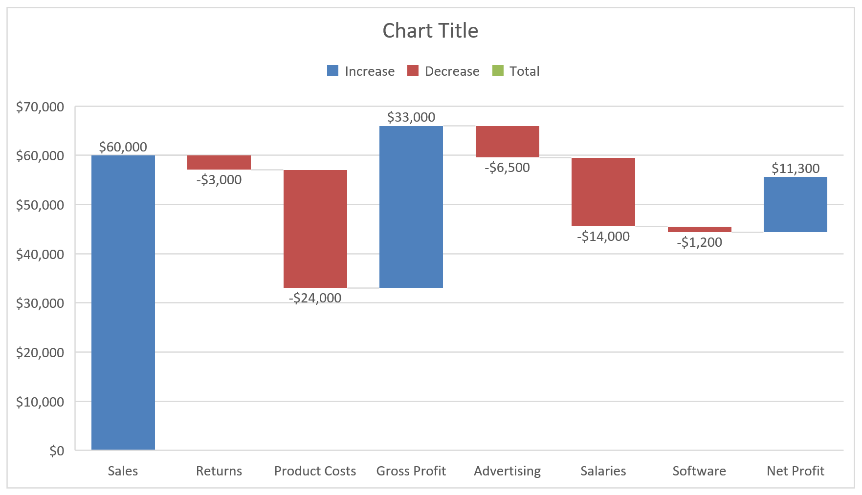
Excel plots Gross Profit as one more increase, so its bar shoots up from where Product Costs ended. Net Profit floats in the same way.

2. Click the Gross Profit bar twice so only that bar is selected, right-click it, and click Set as Total.

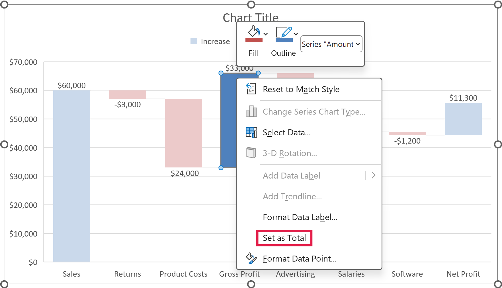
3. Do the same for the Net Profit bar.

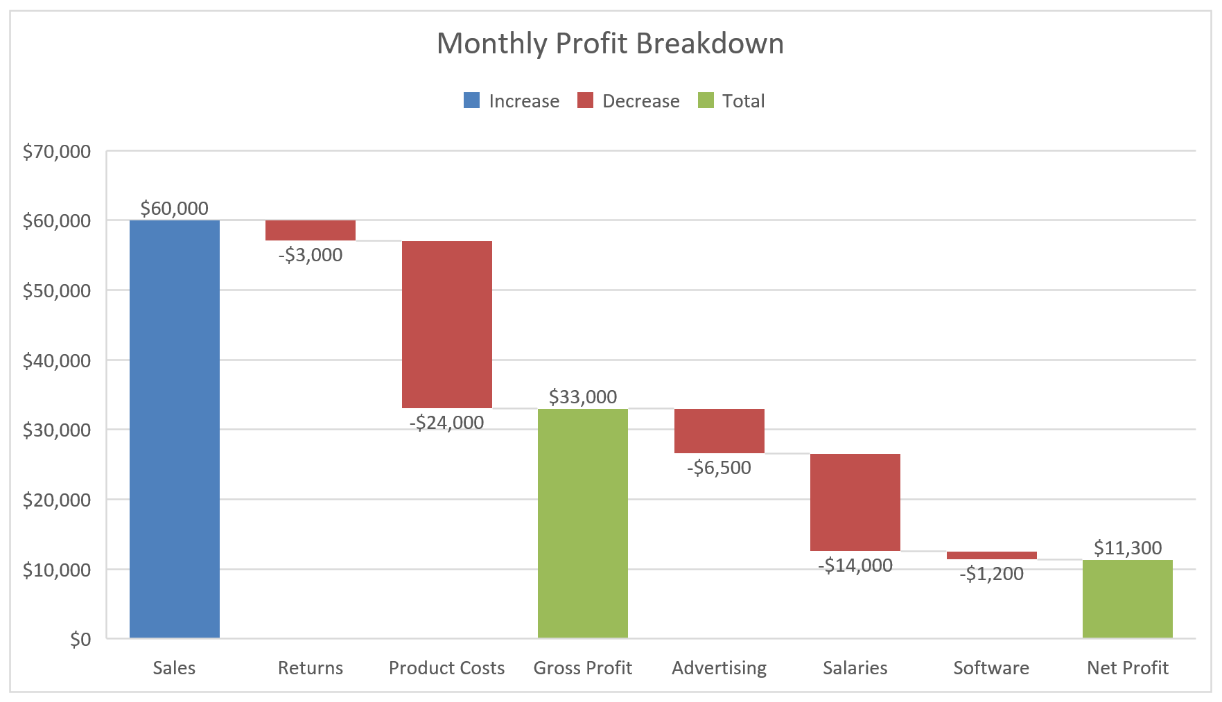
Now Gross Profit and Net Profit both start at zero, so you can see sales drop to gross profit and then to net profit.

Sales stays a change, because it’s money coming in, not a balance carried over from before. And since it’s the first bar, it already starts at zero.

Method 2: Make a Waterfall Chart with a Stacked Column Chart (Excel 2013 and Earlier)

Here’s another way to do this if you’re on Excel 2013, 2010, or an older version that doesn’t have the built-in Waterfall chart. The trick is to fake the floating bars with a stacked column chart.

The idea is to add a helper series called Base that pushes each bar up to the right height, and then make it invisible. Your Increase, Decrease, and Total bars sit on top of that base.

Important: This method works only while the running total stays at zero or above. If it dips below zero, the bars get drawn from the axis instead of floating, and only the built-in chart in Excel 2016 or later handles that data.

We’ll use the same cash flow summary and add four helper columns, Base, Increase, Decrease, and Total, in columns C to F, which split each amount in column B and track the running total.

Setting Up the Helper Columns

The Base values become the invisible bottom part of each bar in the chart. For an increase, the base is the running total so far, so the bar starts where the previous bar ended.

For a decrease, the base is the new, lower total. That way, the bar hangs down from the old total to the new one.

The Starting Balance and Ending Balance bars sit on the baseline, so their base is 0. Type 0 in cells C2 and C9.

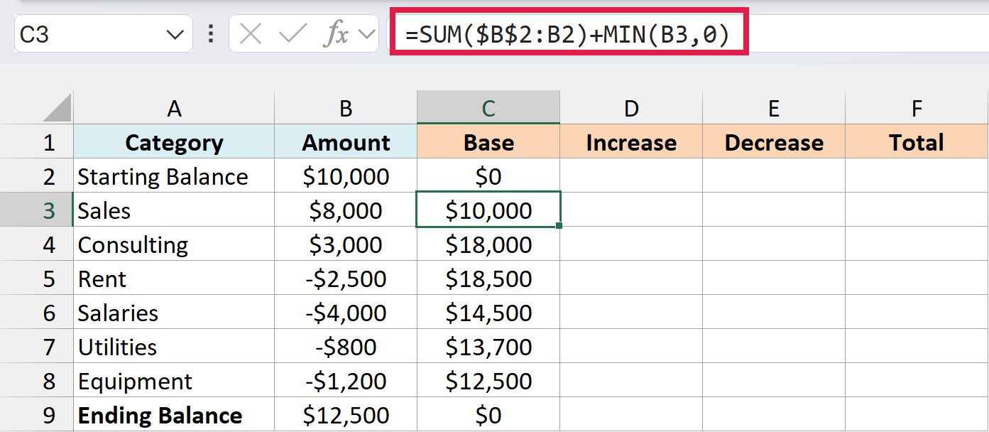
For the rows in between, enter this formula in cell C3 and copy it down to C8:

=SUM($B$2:B2)+MIN(B3,0)

How this formula works:

• SUM($B$2:B2) adds up every amount above the current row. The first reference is locked with $ signs and the second one is not, so the range grows as you copy the formula down.
• MIN(B3,0) returns 0 for an increase, so the bar simply starts at the previous total.
• For a decrease, MIN(B3,0) returns the negative amount. That drops the base down to the new total, so the bar hangs from the old total down to the new one.

Important: Don’t copy the Base formula into C9. The Ending Balance is a total, not a change, but the formula would return the running total of $12,500 there and float that bar up to $25,000.

Next comes the Increase column, which keeps only the amounts that add to your balance. Enter this formula in cell D3 and copy it down to D8:

=MAX(B3,0)

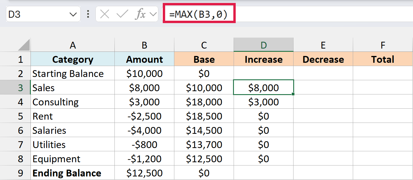
MAX(B3,0) gives you the amount itself when it’s positive and 0 when it’s negative. So Sales and Consulting show up here, and Rent, Salaries, Utilities, and Equipment come through as 0.

Then there’s the Decrease column, which keeps the size of each negative amount. Enter this formula in cell E3 and copy it down to E8:

=-MIN(B3,0)

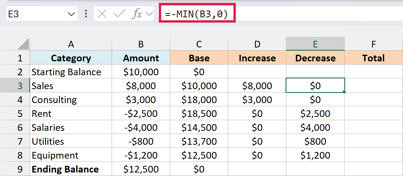
MIN(B3,0) grabs the negative amounts, and the minus sign in front flips them to positive. Chart bars need a positive height, so Rent’s -$2,500 becomes $2,500 here.

Last is the Total column, which holds the two balance bars. Enter =B2 in cell F2 and =B9 in cell F9, so these bars always match the balances in column B.

Fill the remaining helper cells with 0. That means Increase and Decrease on the two balance rows, and Total on the rows in between, so each row has a value in only one of the three bar columns.

Notice how the numbers chain together in the Sales, Consulting, and Rent rows.

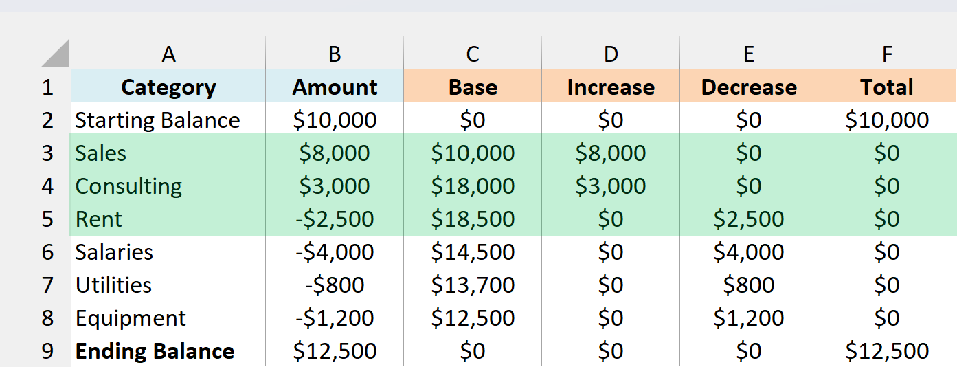
Sales has a base of $10,000 and adds $8,000, so its bar tops out at $18,000, which is exactly where the Consulting bar starts.

Rent works the other way. Consulting took the total to $21,000, and Rent’s base is $18,500 with $2,500 of decrease, so its bar hangs from $21,000 down to $18,500.

Building the Stacked Column Chart

These steps use the names from current versions of Excel. Where Excel 2013 or Excel 2010 looks different, I’ve noted it beside that step.

Here are the steps to turn the helper columns into a waterfall chart:

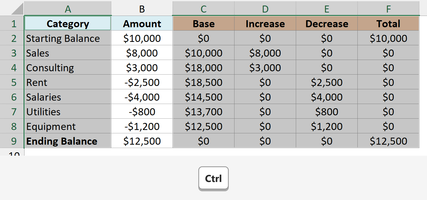
1. Select A1:A9, then hold the Ctrl key and select C1:F9. This picks up the category names and the four helper columns, and skips the amounts in column B.

2. Click the Insert tab, click the Insert Column or Bar Chart icon, and click Stacked Column.

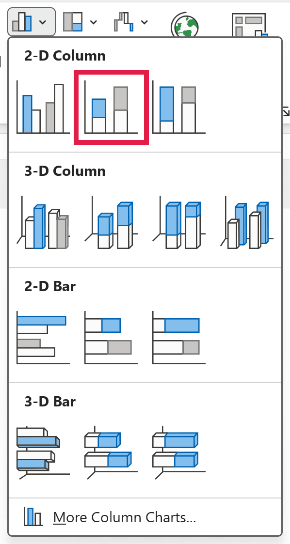
In Excel 2013, this icon is called Insert Column Chart. In Excel 2010, click Column in the Charts group instead.

3. Right-click the Base series (the bottom part of each column), click Format Data Series, and under Fill, select No fill.

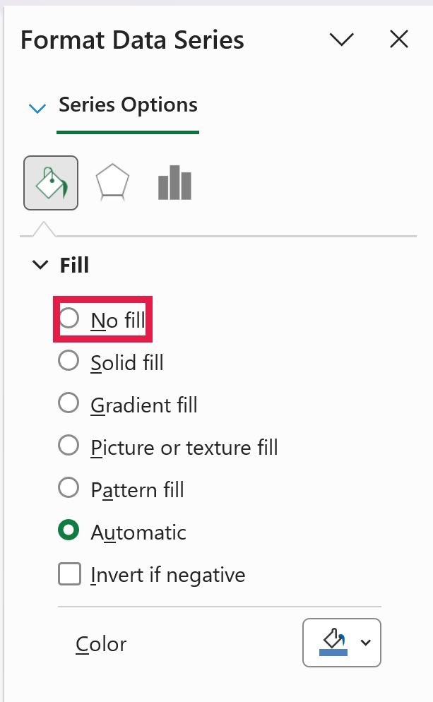
In Excel 2010, Format Data Series opens a dialog box instead of a pane, and No fill is under the Fill tab.

4. Click the legend once, then click the Base entry and press the Delete key. This clears the leftover swatch for a series nobody can see.

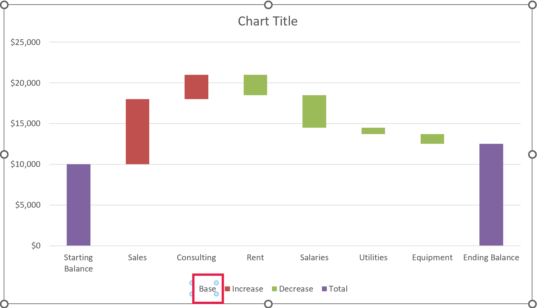
With the base hidden, the Increase, Decrease, and Total bars appear to float, which gives you the waterfall look. Next, give each series its own color.

5. Right-click any Increase bar, click the Fill drop-down, and pick green.

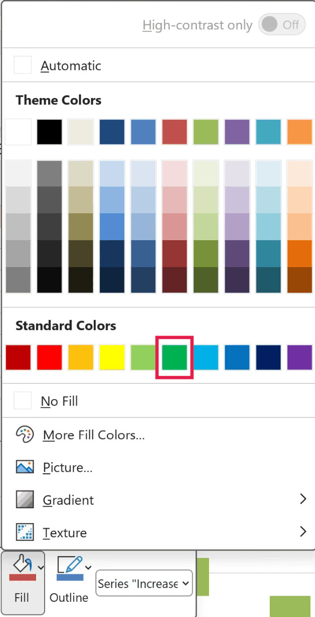
Do the same for the Decrease bars (red) and the Total bars (gray). Since the balances have a series of their own, the legend shows Increase, Decrease, and Total, just like the built-in chart.

6. Click the Chart Title box, select the placeholder text, and type a title, such as Cash Flow for the Quarter.

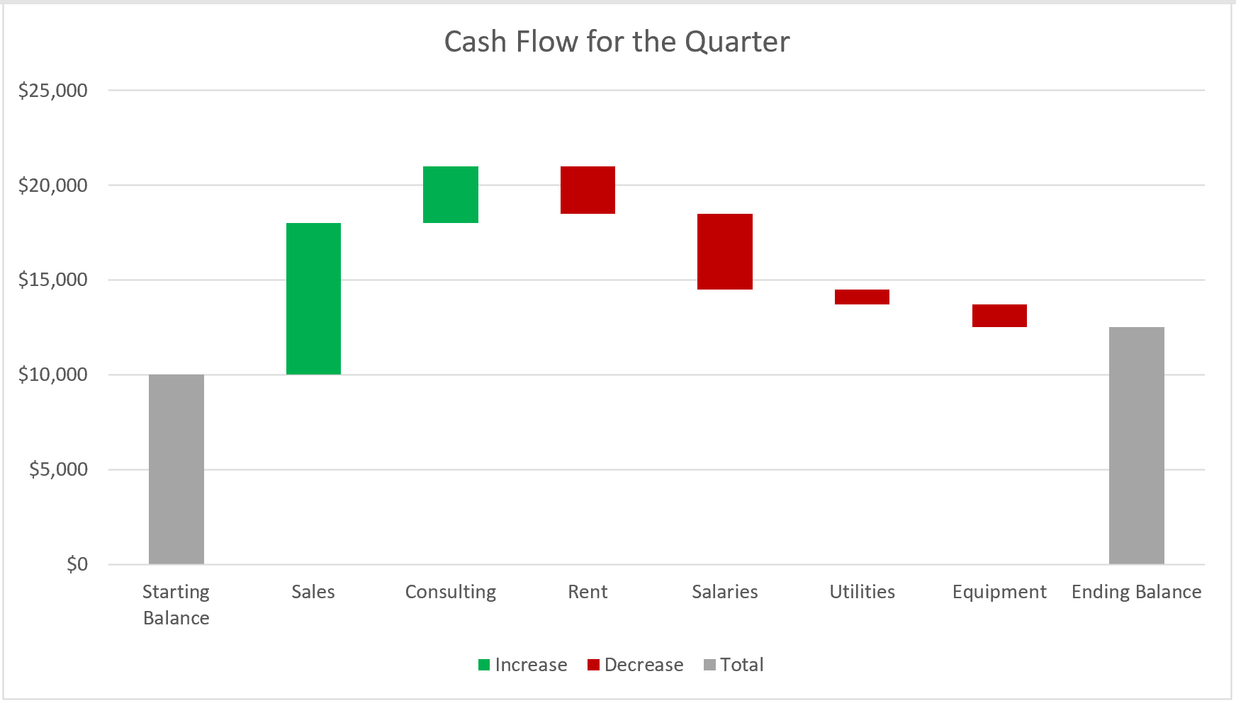
To make the bars wider, right-click any bar, click Format Data Series, and lower the Gap Width (50% works well here).

Unlike the built-in chart, this version has no connector lines between the bars. You can draw them with extra chart series, but that takes a fair bit of extra setup, so I’ve left them out here.

Adding Data Labels to the Stacked Column Chart

A stacked column chart doesn’t add data labels on its own. And when you add them, every series gets labels, including the invisible Base and the zeros in each helper column, so a little cleanup is needed.

Here are the steps to add clean data labels:

1. Click the chart, click the Chart Elements button (the plus icon next to the chart), and check Data Labels.

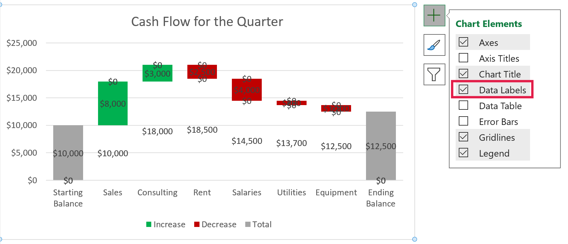
Excel 2010 doesn’t have the Chart Elements button. Click the chart, and on the Layout tab under Chart Tools, click Data Labels and pick Center.

2. Click any label of the Base series (the amounts floating where the invisible base sits) and press the Delete key.

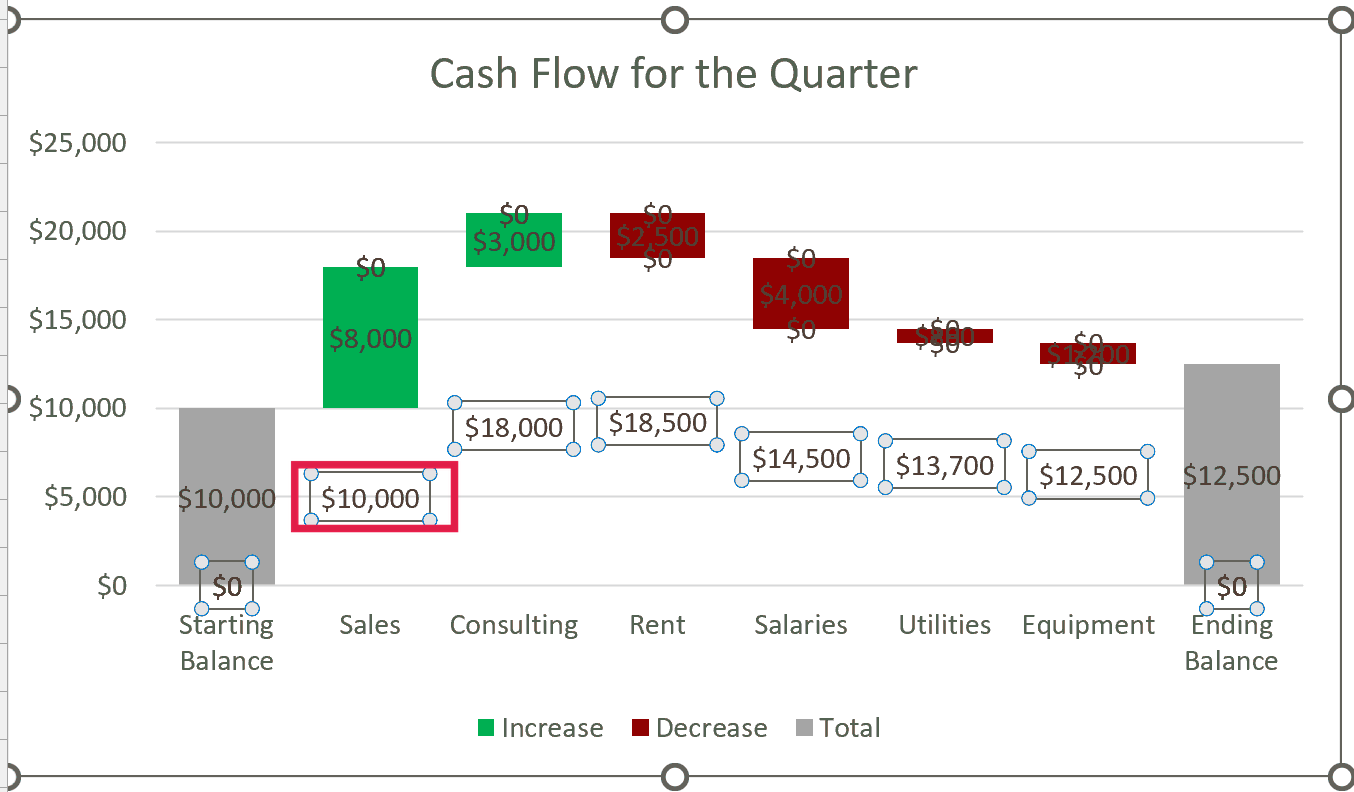
3. Click any Increase label, press Ctrl + 1 to open the Format Data Labels pane, and under Number, select Custom, type $#,##0;;; in the Format Code box, and click Add.

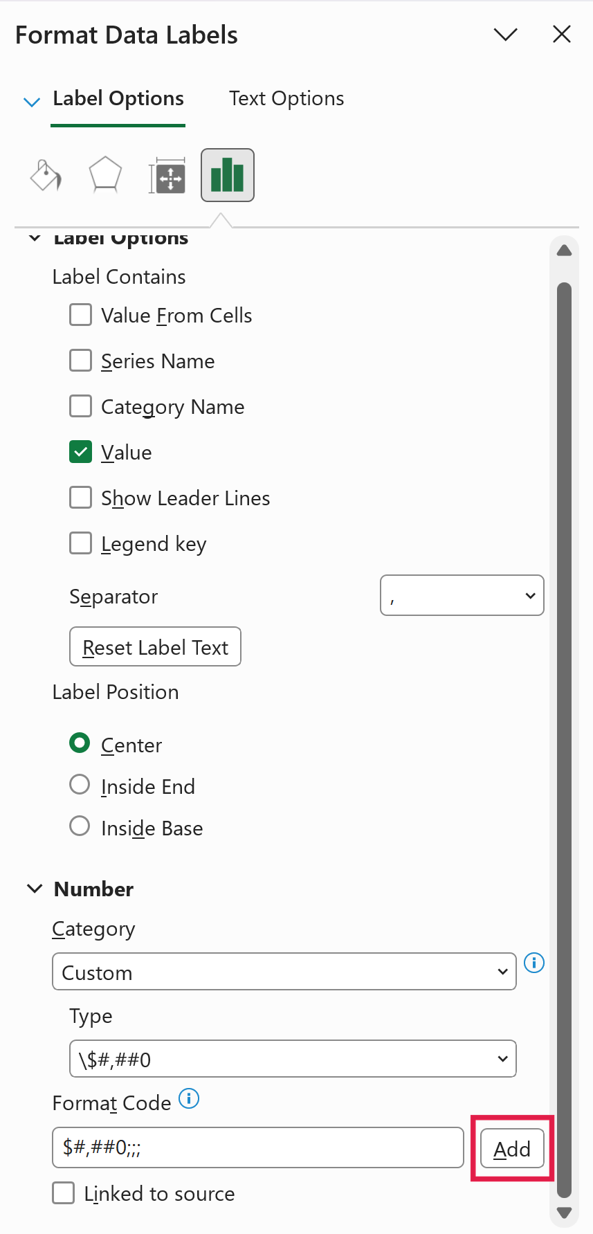
In Excel 2010, Ctrl + 1 opens a Format Data Labels dialog box, and the same Custom format code goes under its Number tab.

In this custom number format, the three semicolons leave the format empty for negative numbers, zeros, and text, so the $0 labels disappear and only the real amounts show.

Repeat this for the Total labels with the same format code. For the Decrease labels, use -$#,##0;;;, which adds the minus sign back so a decrease reads as -$2,500 instead of $2,500.

This method takes more setup than the built-in chart, so use Method 1 whenever your version of Excel has it.

In this article, I showed you how to create a waterfall chart in Excel using the built-in chart type, how to add subtotals to it, and how to build one with a stacked column chart for older versions.

I hope you found this article helpful.

Other Excel Articles You May Also Like:

• How to Make a Chart (Graph) in Excel
• 10 Advanced Excel Charts that You Can Use In Your Day-to-day Work
• How to Create a Sales Funnel Chart in Excel
• Step Chart in Excel – A Step by Step Tutorial
• Add Total Values for Stacked Bar Charts in Excel