

The COUPNUM function in Excel counts how many coupon payments remain between a bond’s settlement date and maturity date. A coupon is the interest payment a bond makes on a regular schedule.
For example, a bond that pays interest twice a year may have five payments left even though it matures in a little over two years. COUPNUM works from the payment schedule, so you don’t have to count those dates yourself.
Below, I’ll show you how to count the remaining payments, compare payment frequencies, and use the count to calculate scheduled coupon cash.
Follow along with the example file
COUPNUM Function Examples.xlsx
COUPNUM Function Syntax
Here is the syntax of the COUPNUM function:
=COUPNUM(settlement, maturity, frequency, [basis])
- settlement: The date the bond purchase settles. This is the starting date for the count.
- maturity: The date the bond matures, when its principal is due to be repaid. The regular coupon schedule works backward from this date.
- frequency: The number of coupon payments each year. Use 1 for annual payments, 2 for semiannual payments, or 4 for quarterly payments.
- basis: An optional code for the day-count convention. If you leave it out, Excel uses 0, which means US (NASD) 30/360.
A day-count convention specifies how to count days for bond calculations. A 30/360 convention uses standardized 30-day months and a 360-day year, while actual-day conventions count calendar days in the period.
The other basis choices are 1 for actual/actual, 2 for actual/360, 3 for actual/365, and 4 for European 30/360. The part after the slash describes the year length used: the actual year length, 360 days, or 365 days.
Use the convention specified for the bond. The basis argument doesn’t set how often payments happen; the frequency argument does that.
Excel truncates all four arguments to integers. That means time portions of dates are ignored, and decimal frequency or basis values aren’t rounded to the nearest choice.
The COUPNUM function is available in Excel 2016 and later, including Microsoft 365 and current Mac versions. The spilling examples below require dynamic arrays, available in Microsoft 365, Excel 2024, and Excel 2021; they were tested in Microsoft 365 for Windows.
When to Use the COUPNUM Function
Use this function when you need to:
- Count the regular coupon payments remaining on a bond.
- Compare annual, semiannual, and quarterly payment schedules.
- See how the count changes as the settlement date moves forward.
- Calculate scheduled coupon receipts when you also know each payment’s amount.
Let’s start with one bond, then work through the comparisons.
Example 1: Count the Remaining Coupon Payments
Let’s start with a bond that pays interest twice a year.
Below are its settlement date, maturity date, payment frequency, and basis, and I want to get the remaining coupon count in cell B6.
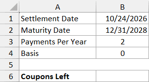
Enter this formula in cell B6 and press Enter:
=COUPNUM(B1,B2,B3,B4)
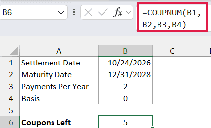
The formula returns 5. Settlement is October 24, 2026, maturity is December 31, 2028, and the frequency of 2 means there are two coupon payments each year.
Working backward from maturity, the five remaining payment dates are December 31, 2026; June 30 and December 31, 2027; and June 30 and December 31, 2028. The payment at maturity is included in the count.
The first of these payments is only a little over two months after settlement, but it still counts as one payment. COUPNUM returns a whole number of coupons, not a fractional number of years.
Important: The settlement date must be earlier than maturity, or COUPNUM returns #NUM!, including when the two dates are equal. It also returns #NUM! for an unsupported frequency or a basis outside 0 through 4.
The dates must be real Excel dates. Invalid dates can produce #VALUE!, and changing a text cell’s number format to Date doesn’t convert the text into a date value.
The example file already contains real dates. If you’re building your own inputs, the DATE function lets you create a date from separate year, month, and day values without relying on how Excel interprets typed date text.
The screenshots use month/day/year formatting. Your date display may differ with your regional settings, but the calculation uses the underlying date values.
Example 2: Compare Three Coupon Payment Frequencies
Now let’s keep the dates the same and change how often the bond pays interest.
Below are annual, semiannual, and quarterly schedules, and I want to compare their remaining coupon counts in column C.

Enter this formula in cell C2 and press Enter:
=COUPNUM(F1,F2,B2:B4+0)
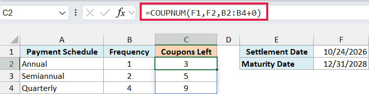
One formula returns all three results: 3 annual payments, 5 semiannual payments, and 9 quarterly payments. The results spill into the cells below C2 automatically, so there’s no need to copy the formula down.
The formula uses the dates in F1 and F2 for every calculation. The frequency changes with each value in B2:B4, while the omitted basis argument defaults to 0.
The +0 after B2:B4 matters here. COUPNUM can return #VALUE! when given a plain range for this argument; adding zero turns the range into an array of numbers that the function can evaluate, without changing those numbers.
Keep the spill cells below C2 empty before entering the formula. If something blocks the results, Excel returns #SPILL!, so clear the cells in the intended output area.
Only the three listed frequencies are supported. A monthly schedule with frequency 12 isn’t valid for COUPNUM, even though other financial calculations may use 12 payments per year.
If you’re using Excel 2019 or earlier, enter the following formula in cell C2 and copy it down to C4:
=COUPNUM($F$1,$F$2,B2)
The dollar signs keep the dates fixed while the frequency reference changes for each row.
Example 3: Compare Different Settlement Dates
The count also changes when you move the settlement date across a coupon date.
Below are six possible settlement dates for the same semiannual bond, and I want to see the remaining coupon count for each date in column B.
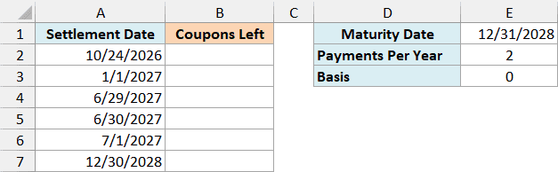
Enter this formula in cell B2 and press Enter:
=COUPNUM(A2:A7+0,E1,E2,E3)
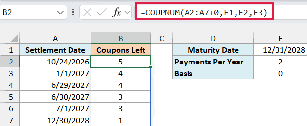
The results are 5, 4, 4, 3, 3, and 1. Each date in A2:A7 is tested against the same maturity, frequency, and basis in E1:E3, with the same +0 adjustment used in the previous example.
Look at June 29 and June 30, 2027. On June 29, the June 30 coupon is still ahead, so the count is 4; on June 30 itself, the count drops to 3.
COUPNUM counts the scheduled coupon dates after settlement, so it doesn’t include a coupon date equal to settlement. Moving settlement forward to July 1 leaves the count at 3 because no additional coupon date has passed.
The final row returns 1 even though settlement is only one day before maturity. The final coupon is still ahead, so the count hasn’t reached zero.
If you’re using Excel 2019 or earlier, enter the following formula in cell B2 and copy it down to B7:
=COUPNUM(A2,$E$1,$E$2,$E$3)
This keeps the bond’s terms fixed and uses the settlement date on each row.
Example 4: Calculate Remaining Coupon Cash
Once you know the number of payments, you can multiply it by the amount of each coupon.
Below are six fictional bond holdings with face values, annual coupon rates, and maturity dates, and I want the remaining payment counts in column E and scheduled coupon cash in column F.
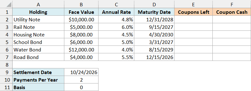
All six holdings use the same settlement date and pay interest twice a year. The annual rate is the bond’s coupon rate, and face value is the principal amount used to calculate interest.
First, enter this formula in cell E2 and press Enter:
=COUPNUM(B9,D2:D7+0,B10,B11)
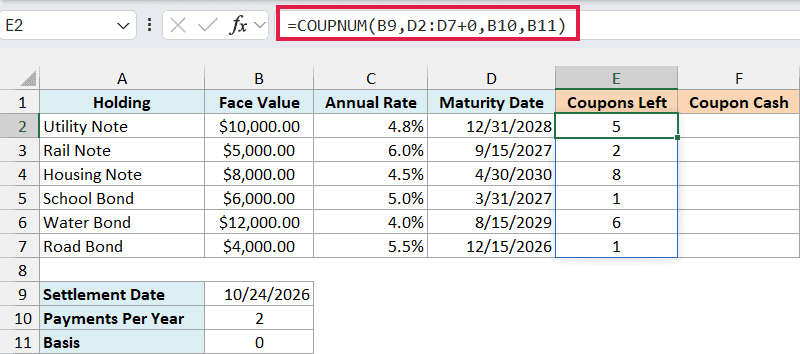
The formula spills the six coupon counts into column E: 5, 2, 8, 1, 6, and 1. It uses each maturity date in column D with the shared settlement date, frequency, and basis below the table.
Next, enter this formula in cell F2 and press Enter:
=B2:B7*C2:C7/$B$10*E2#
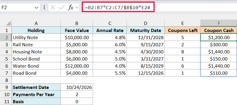
How this formula works:
B2:B7*C2:C7multiplies each face value by its annual coupon rate to get one year’s coupon amount.- Dividing by
$B$10splits that amount into two equal payments per year. E2#refers to all the coupon counts spilled from E2. Multiplying by those counts gives the remaining scheduled coupon cash for each holding.
For the Utility Note, $10,000 multiplied by 4.8% gives $480 a year. Each semiannual coupon is $240, and five remaining payments give $1,200.
The six results are $1,200, $300, $1,440, $150, $1,440, and $110. They are the total scheduled coupon receipts from settlement through maturity under these regular payment schedules.
Important: Coupon cash isn’t investment profit or present value. This calculation excludes principal repayment and accrued-interest adjustments, assumes regular equal coupons, and assumes the bond isn’t redeemed early and all scheduled payments are made.
If you’re using Excel 2019 or earlier, enter the following formula in cell E2 and copy it down to E7:
=COUPNUM($B$9,D2,$B$10,$B$11)
Then enter this formula in cell F2 and copy it down to F7:
=B2*C2/$B$10*E2
These calculate the same results one row at a time, without spill references.
In this article, I showed you how to use COUPNUM to count remaining payments, compare schedules, and calculate scheduled coupon cash. I hope you found it helpful.
Other Excel Articles You May Also Like:
