

If you have numbers with decimals and you just want the whole number part, the INT function in Excel is the quickest way to get it.
It rounds a number down to the nearest whole number, so 4.85 becomes 4 and a date-time value becomes just the date. It works the same way on a single cell or a whole column.
In this article, I’ll show you how to use the INT function in Excel, what it does with negative numbers, and how it’s different from TRUNC and ROUNDDOWN.
Follow along with the example file
INT Function Examples.xlsx
INT Function Syntax
The INT function takes one number and rounds it down to the nearest integer (a whole number with no decimals).
=INT(number)
Here’s what the argument means:
- number – the number you want to round down to a whole number. This can be a value you type in, a cell reference, or a range of cells.
One thing to keep in mind: INT always rounds down, toward the lower number. For positive numbers that just means it drops the decimals. For negative numbers it behaves a little differently, and I’ll cover that in Example 2.
Example 1: Get the Whole Number Part of a Decimal
The most common use is the simplest one. You have a column of prices with decimals, and you want just the whole-dollar part of each one.
Below I have a list of item prices in column A, and I want to get the whole number for each price in column B.
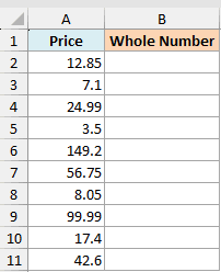
In Excel 365, you can point INT at the entire range in one go, and the results spill down the column automatically.
=INT(A2:A11)
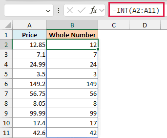
You type this single formula in cell B2 and press Enter. Excel fills the whole result range for you, so there’s no need to copy the formula down.
For example, 12.85 becomes 12 and 7.10 becomes 7. INT keeps the whole number and drops everything after the decimal point.
Pro Tip: If you’re on an older version of Excel that doesn’t spill, type =INT(A2) in cell B2 and copy it down the column. You get the same result, one cell at a time.
Example 2: What INT Does With Negative Numbers
This is the part that trips people up, so it’s worth its own example.
Below I have a list of temperature readings in column A, some of them below zero, and I want the whole number for each one in column B.
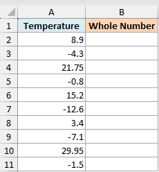
Here’s the formula, pointed at the whole range so it spills down column B:
=INT(A2:A11)
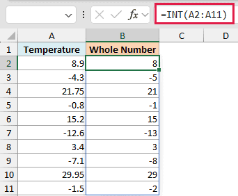
For the positive values it works as you’d expect. 8.90 becomes 8.
But look at -4.30. INT gives you -5, not -4. That’s because INT rounds down to the lower number, and -5 is lower than -4.30 on the number line.
So for a negative number, INT moves further away from zero. If you actually wanted -4 here (just chopping off the decimals), that’s a job for TRUNC, which I cover further down.
Example 3: Extract the Date From a Date and Time
Excel stores a date and time as a single number. The part before the decimal is the date, and the part after the decimal is the time.
That means INT is perfect for pulling just the date out of a date-time value, because rounding down to the whole number leaves you with the date and drops the time.
Below I have a column of order timestamps in column A, each with a date and a time, and I want just the date in column B.
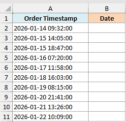
Here’s the formula:
=INT(A2:A11)
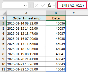
Once you enter it, the result will show as a number. Select the result cells, and from the Home tab set the format to Short Date so the whole numbers display as dates.
Pro Tip: INT strips the time by rounding the value down, so the date it returns is always correct. This is a clean way to group timestamps by day.
Follow along with the example file
INT Function Examples.xlsx
Example 4: Get the Time Part From a Date and Time
You can flip the last example around. If INT gives you the date (the whole number part), then subtracting INT from the original value leaves you with just the time (the decimal part).
Below I have the same order timestamps in column A, and this time I want just the time in column B.
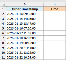
Here’s the formula:
=A2:A11-INT(A2:A11)
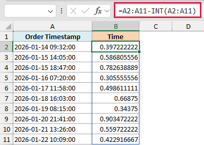
The value minus its own whole number part is exactly the leftover decimal, which is the time. Format the result cells as Time from the Home tab and you’ll see the clock value for each order.
If you want to work with that time as a plain number instead, see how to convert time to a decimal.
Example 5: Get the Age From a Date of Birth
To calculate age in complete years, use DATEDIF with “Y”. YEARFRAC‘s default financial US 30/360 day count can reach a whole year before the birthday, so wrapping it in INT can give the wrong age.
Below I have a list of names with their dates of birth in column B, and I want each person’s age in whole years in column C.
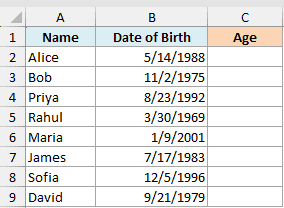
Here’s the formula:
=DATEDIF(B2,TODAY(),"Y")
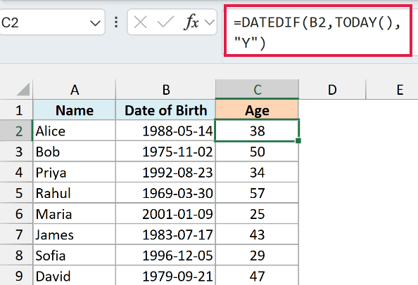
Here’s how this formula works:
- B2 contains the date of birth, and TODAY() supplies today’s date.
- “Y” tells DATEDIF to return the number of complete years between those dates.
The INT/YEARFRAC approach uses this formula with the date of birth in cell B2:
=INT(YEARFRAC(B2,TODAY()))
For someone born on March 31, 2000, this formula returns an age of 21 on March 30, 2021. DATEDIF returns 20, then 21 on March 31, 2021.
Copy this formula down column C to get the age for everyone in the list. Since the TODAY function updates on its own, these ages stay current every time the sheet recalculates.
Example 6: INT vs TRUNC vs ROUNDDOWN
INT isn’t the only function that gets rid of decimals. TRUNC and ROUNDDOWN do a similar job, and for positive numbers all three give you the same answer. The difference shows up with negative numbers.
Below I have a few sample values in column A, and I’ve run each one through INT, TRUNC, and ROUNDDOWN so you can compare.
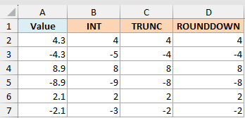
Here’s what each one does:
- INT rounds down to the lower whole number. On a negative number that means moving away from zero, so INT(-4.3) gives -5.
- TRUNC just chops off the decimals and keeps the sign, so TRUNC(-4.3) gives -4.
- ROUNDDOWN also rounds toward zero, so ROUNDDOWN(-4.3, 0) gives -4, and it lets you pick how many decimal places to keep.
For 4.3, all three return 4. For -4.3, INT gives -5 while TRUNC and ROUNDDOWN give -4.
So the rule of thumb is simple. If you want the true lower whole number, use INT. If you just want to cut off the decimals and leave the sign alone, use TRUNC or ROUNDDOWN.
Things to Keep in Mind
A few quick points that will save you some head-scratching:
- INT only rounds down, never up. It has no option to round to the nearest whole number. If you want normal rounding, use the ROUND function instead.
- Negative numbers go to the lower value. INT(-2.1) is -3, not -2. If that’s not what you want, reach for TRUNC.
- Date results show as a number at first. When you use INT on a date-time value, apply a Date format to the result so it reads as a date instead of a serial number.
- INT takes just one argument. If you need to control decimal places, that’s ROUNDDOWN, not INT.
INT is one of those small functions you’ll reach for again and again once it’s in your toolkit, whether you’re cleaning up prices or pulling dates out of timestamps.
I hope you found this Excel tutorial helpful.
Other Excel Articles You May Also Like:
- How to Use Excel MOD Function
- How to Remove Time from Date/Timestamp in Excel
- How to Round to the Nearest Integer or Multiple of 0.5 / 5 / 10 in Excel
- How to Calculate Age in Excel using Formulas + FREE Calculator Template
- HOUR in Excel
- ROUNDUP in Excel
- FLOOR Function in Excel
- FLOOR.MATH Function in Excel
