

The MUNIT function creates an identity matrix, also called a unit matrix. This is a square grid with 1s running diagonally from the top-left to the bottom-right and 0s everywhere else.
If you need that pattern for a matrix calculation, you don’t have to type the numbers yourself. Give MUNIT the size of the matrix, and it creates the whole grid.
In this tutorial, I’ll show you how to create an identity matrix, change its diagonal values, and use it in two calculations.
Follow along with the example file
MUNIT Function Examples.xlsx
MUNIT Function Syntax
Here is the syntax of the MUNIT function:
=MUNIT(dimension)
- dimension is required. It specifies both the number of rows and the number of columns in the matrix.
A dimension of 4 creates a 4-by-4 matrix, so the result contains 16 numbers. You can enter the dimension directly or refer to a cell containing it.
Use a positive whole number for the dimension. If you supply a decimal such as 2.9, Excel drops the decimal part and creates a 2-by-2 matrix; a dimension of zero or less returns a #VALUE! error.
The MUNIT function is available in Excel 365, 2024, 2021, 2019, and 2016, including current Mac versions. Excel 365, 2024, and 2021 spill the matrix automatically; older versions need array entry.
When to Use the MUNIT Function
Use this function when you need to:
- Create an identity matrix of a specified size.
- Build a square matrix with the same number along its diagonal.
- Demonstrate how an identity matrix behaves in matrix multiplication.
- Select the main diagonal of a square grid for a calculation.
Let’s start with the identity matrix itself, then use that pattern in the other examples.
Example 1: Create an Identity Matrix in Excel
On the Identity Matrix sheet, the dimension in cell B1 is 4, and I want to create an identity matrix starting in column D.
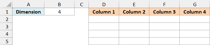
Enter the following formula in cell D2 and press Enter:
=MUNIT(B1)
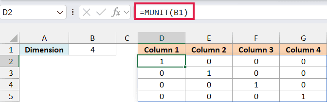
The formula reads the 4 in B1 and fills D2:G5 with a 4-by-4 identity matrix. The four diagonal cells contain 1, while every other cell contains 0.
This is called a spill: you enter one formula, and Excel places its results into the neighboring cells. To change the formula, select D2, which is the top-left cell of the result.
Changing B1 to 3 gives you a 3-by-3 matrix instead. The size changes automatically, so you don’t need to rewrite the formula.
Important: The cells needed by the matrix must be empty before you enter the formula. If something blocks the output, Excel returns a #SPILL! error; move the blocking content or place the formula where the entire matrix fits.
In Excel 2019 or 2016, select D2:G5, type the formula below, and confirm it with Ctrl+Shift+Enter:
=MUNIT(B1)
Those older versions use the selected output area instead of resizing it automatically. If you change the dimension, select an output area of the new size and enter the array formula again.
Example 2: Create a Constant Diagonal Matrix
An identity matrix always has 1s on its main diagonal. If you need a different number there, multiply the matrix by that number.
On the Scaled Diagonal sheet, B1 contains the dimension 3 and B2 contains the diagonal value 7, and I want the resulting matrix to start in column D.
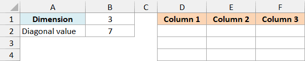
Enter the following formula in cell D2 and press Enter:
=B2*MUNIT(B1)
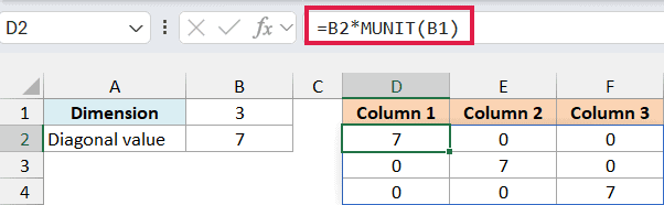
The MUNIT function first creates a 3-by-3 identity matrix. Multiplying it by B2 changes each diagonal 1 to 7, while the zeros stay zero.
The result fills D2:F4. You can change B2 to another number to change all three diagonal values together.
This is a diagonal matrix, but it is no longer an identity matrix because its diagonal values aren’t 1.
In Excel 2019 or 2016, select D2:F4, enter the formula below, and confirm it with Ctrl+Shift+Enter:
=B2*MUNIT(B1)
Example 3: Multiply by an Identity Matrix
Multiplying a number by 1 leaves it unchanged. An identity matrix plays a similar role in matrix multiplication, which combines rows from one matrix with columns from another.
On the Matrix Multiplication sheet, the table contains notebook and pen quantities for three supply packs, and I want to show the identity-multiplication result in columns E and F.

Enter the following formula in cell E2 and press Enter:
=MMULT(B2:C4,MUNIT(COLUMNS(B2:C4)))
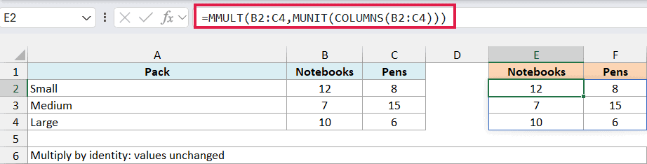
The output in E2:F4 matches the original quantities: 12 and 8, 7 and 15, then 10 and 6. That’s the identity rule at work.
How this formula works:
- The COLUMNS function counts the two columns in B2:C4.
- The MUNIT function uses that count to create a 2-by-2 identity matrix.
- The MMULT function multiplies the original 3-by-2 matrix by that identity matrix, returning the original values.
The size matters here: the first matrix has two columns, so the second matrix must have two rows. Using the COLUMNS function gives the identity matrix the right size without typing a fixed dimension.
For the first pack, the first output is 12 times 1 plus 8 times 0, which gives 12. The second is 12 times 0 plus 8 times 1, which gives 8.
This example demonstrates a matrix property. If you only want to copy the quantities elsewhere, a direct reference is simpler and avoids doing matrix multiplication.
Important: The MMULT function requires numbers in both input arrays. Blank cells or text in B2:C4 cause a #VALUE! error, so make sure the quantities are numeric.
In Excel 2019 or 2016, select E2:F4, enter the formula below, and confirm it with Ctrl+Shift+Enter:
=MMULT(B2:C4,MUNIT(COLUMNS(B2:C4)))
Example 4: Sum the Main Diagonal
You can also use the 1s and 0s from MUNIT to keep diagonal values and ignore the rest. Let’s use a library returns table to see why that can be useful.
On the Diagonal Total sheet, rows identify the borrowing branch and columns identify the return branch, and I want the number of books returned to their original branch in cell B6.
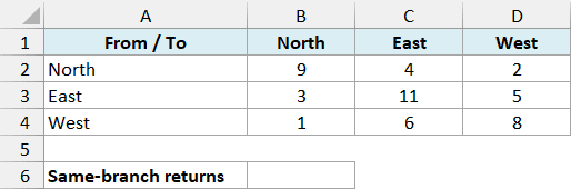
Enter the following formula in cell B6 and press Enter:
=SUMPRODUCT(B2:D4,MUNIT(ROWS(B2:D4)))
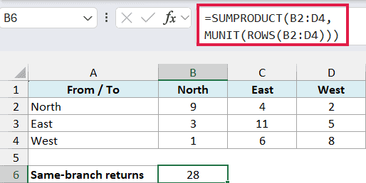
The result is 28: 9 books for North, 11 for East, and 8 for West. These are the cells where the borrowing branch and return branch are the same.
How this formula works:
- The ROWS function counts the three rows in B2:D4.
- The MUNIT function creates a 3-by-3 matrix with 1s on the main diagonal and 0s elsewhere.
- The SUMPRODUCT function multiplies each return count by the corresponding 1 or 0, then adds the products. Only the three diagonal values contribute to the total.
Unlike the earlier examples, this formula returns a single number. The matrix is used inside the calculation, so the SUMPRODUCT function needs only cell B6 and works with a normal Enter in the older versions too.
Important: Keep the data range square and the branch names in the same order across the top and down the side. If the order differs, the main diagonal won’t represent same-branch returns.
For three permanently fixed cells, a direct sum is simpler. This example shows a diagonal-selection pattern you can reuse with another square grid by updating the B2:D4 references to cover that grid.
So you can use MUNIT on its own to create an identity matrix, or use its diagonal pattern inside another calculation. Match the dimension to the size your calculation needs, and leave enough room when the result spills onto the sheet.
Other Excel Articles You May Also Like:
