

The MINVERSE function in Excel returns the inverse of a square matrix. You give it a grid of numbers with the same number of rows and columns, and it returns another grid of the same size.
On its own, an inverse matrix is mostly something you meet in a math or statistics class. Paired with the MMULT function, though, it lets you solve a set of equations with several unknowns in a single formula.
The catch is that not every matrix has an inverse, and Excel doesn’t always warn you when it doesn’t. I’ll show you how to spot that too.
Follow along with the example file
MINVERSE Function Examples.xlsx
MINVERSE Function Syntax
Here is the syntax of the MINVERSE function:
=MINVERSE(array)
- array – the square matrix you want to invert. This can be a range of cells (like A2:C4), an array constant (like {5,2;7,3}), or a named range. It’s the only argument, and it’s required.
The array has to be square, with the same number of rows and columns. If it isn’t, MINVERSE returns a #VALUE! error.
Every cell in the array also has to hold a number. A blank cell or a cell with text gives you a #VALUE! error, because MINVERSE doesn’t treat a blank as zero.
The MINVERSE function works in all Excel versions, including Excel for Microsoft 365, Excel 2024, 2021, 2019, 2016, Excel for Mac, and Excel for the web.
When to Use the MINVERSE Function
Use this function when you need to:
- Find the inverse of a 2×2, 3×3, or larger matrix.
- Solve a set of equations with two or more unknowns, together with the MMULT function.
- Undo a matrix multiplication, such as decoding numbers that were scrambled with a key matrix.
- Check your matrix math, since a matrix multiplied by its inverse should give the identity matrix.
Let me show you some practical examples of how to use MINVERSE.
Example 1: Find the Inverse of a 2×2 Matrix
Let’s start with a simple example.
Below I have a 2×2 matrix, and I want to get its inverse in columns D and E.
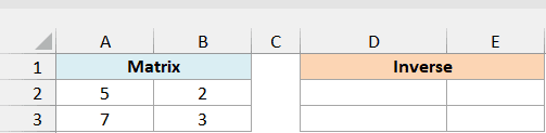
Here is the formula:
=MINVERSE(A2:B3)
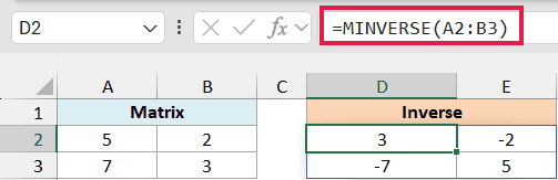
You enter this one formula in D2, and it returns all four values of the inverse: 3, -2, -7, and 5. The results spill into D2:E3, so those cells need to be empty, or you’ll see a #SPILL! error instead.
For a 2×2 matrix, the inverse comes from a simple rule. Swap the two numbers on the diagonal, flip the sign of the other two, and divide everything by the determinant (5×3 – 2×7, which is 1 here).
Since the determinant is 1, this inverse is all whole numbers. Most matrices give you decimals, as you’ll see in the next example.
If you’re using Excel 2019 or earlier, select D2:E3 first, type the below formula, and press Control + Shift + Enter instead of Enter:
=MINVERSE(A2:B3)
Excel adds the curly brackets around the formula by itself. If you press only Enter in those versions, you get just the top-left value (3), and the same goes for every MINVERSE formula in this article.
Example 2: Inverse of a 3×3 Matrix in Excel
Now let’s try a bigger matrix.
Below I have a 3×3 matrix, and I want to get its inverse in columns E to G.
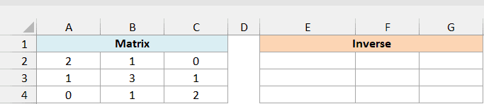
Here is the formula:
=MINVERSE(A2:C4)
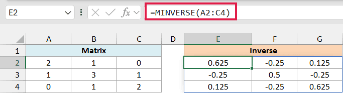
This returns a 3×3 block of results in E2:G4, the same size as the matrix. The first row of the inverse is 0.625, -0.25, and 0.125.
This time the values are decimals. The determinant of this matrix is 8, so every value in the inverse works out to a fraction of 8 (0.625 is 5/8, and -0.25 is -2/8).
Example 3: Check the Inverse With MMULT (Identity Matrix)
Here’s a quick way to check that an inverse is right.
Below I have another 3×3 matrix, and I want to multiply it by its own inverse in columns E to G, which should give the identity matrix if MINVERSE got it right.

Here is the formula:
=MMULT(A2:C4,MINVERSE(A2:C4))

The identity matrix is a grid with 1s running down the diagonal and 0s everywhere else. That’s what you get whenever you multiply a matrix by its inverse.
The diagonal does show 1s here, but some of the 0s show up as tiny numbers like -5.55112E-17. That’s -0.0000000000000000555, a leftover from the way Excel stores decimal numbers, and not a mistake in the inverse.
Excel keeps about 15 to 16 digits of precision, so these leftovers show up a lot with matrix math. They look odd, and they also mean a cell like E3 isn’t exactly zero.
So a check like =E3=0 returns FALSE, even though the value should be 0.
To clean them up, wrap the formula in ROUND:
=ROUND(MMULT(A2:C4,MINVERSE(A2:C4)),10)

The ROUND function rounds every value to 10 decimal places. The leftovers are far smaller than that, so they become exact 0s, and you get a clean identity matrix in I2:K4.
Ten decimal places is a safe choice for everyday matrices. Anything from about 6 to 12 works too, since the leftovers sit way down around the 16th decimal place.
Example 4: Solve a System of Equations Using MINVERSE and MMULT
Now let’s use MINVERSE to solve a real problem.
Below I have three workouts with the minutes spent running, cycling, and swimming, along with the calories burned in each, and I want to get the calories burned per minute for each activity in column H.

Here is the formula:
=MMULT(MINVERSE(B2:D4),E2:E4)

This returns 11 calories per minute for running, 8 for cycling, and 9 for swimming, in the same order as the activity columns. You can check it against Monday: 30×11 + 20×8 + 10×9 comes to 580, which matches.
Each workout is really an equation with three unknowns, one rate per activity. MINVERSE inverts the 3×3 grid of minutes, and multiplying that inverse by the calories in E2:E4 with the MMULT function solves all three equations at once.
The order inside MMULT matters. MINVERSE comes first and the totals come second, because MMULT needs the first array’s columns to match the second array’s rows.
If you swap them, like =MMULT(E2:E4,MINVERSE(B2:D4)), a 1-column range meets a 3-row inverse, and you get a #VALUE! error.
Example 5: Decode a Secret Message by Undoing MMULT
This next one is a fun way to see what an inverse really does.
Below I have a secret message that was turned into numbers and scrambled with a 2×2 key, and I want to decode it back into letters in columns G and H.
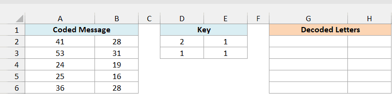
Here’s how the message was coded. Each letter became its position in the alphabet (A=1, B=2, and so on up to Z=26), and each pair of letters was multiplied by the key (2 and 1 in the first row, 1 and 1 in the second) with MMULT.
For example, the first pair is M and O, which is 13 and 15. Multiplied by the key, that gives 2×13 + 15 = 41 and 13 + 15 = 28, which is the first row of the coded message.
Here is the formula that decodes it:
=CHAR(64+ROUND(MMULT(A2:B6,MINVERSE(D2:E3)),0))
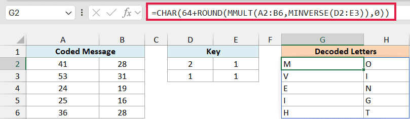
This returns MO, VI, EN, IG, and HT. Read across the rows, the message is MOVIE NIGHT.
How this formula works:
- MINVERSE(D2:E3) returns the inverse of the key, which undoes whatever the key did.
- MMULT(A2:B6, …) multiplies each coded pair by that inverse, so 41 and 28 turn back into 13 and 15.
- ROUND(…, 0) makes sure every result is a whole number.
- CHAR(64+…) turns each number into a letter. 64 + 13 is 77, and CHAR(77) is M.
The ROUND part matters more than it looks. The CHAR function drops any decimals, so a tiny leftover like 12.9999999 (the kind you saw in Example 3) would become the letter L instead of M.
Example 6: Spot a Matrix That Has No Inverse
Let’s finish with a trap that MINVERSE won’t always warn you about.
Below I have three pizza party orders with the number of pizzas, sodas, and salads in each and the total paid, and I want to work out the price of each item in column H.

Here is the formula:
=MMULT(MINVERSE(B2:D4),E2:E4)

This returns $0.00 for a pizza and $16.00 each for a soda and a salad. There’s no error, but the answer is clearly wrong, since a free pizza with $16 sodas and salads would make Friday’s order $64, not $37.
The problem is the Sunday order. It’s exactly Friday’s order plus Saturday’s order (3 pizzas, 7 sodas, 3 salads, and $71), so it adds no new information.
That leaves two real equations for three unknown prices, which means there’s no single answer. Pizza at $12, soda at $2, and salad at $7 fits all three orders, but so does $10, $5, and $2.
A matrix like this has no inverse. MINVERSE does return a #NUM! error for some of these, but here tiny rounding leftovers make the matrix look barely invertible, so you get made-up numbers instead.
Which of the two you get depends on the exact numbers in the matrix. Here a quick check against Friday’s order gave it away, but in a bigger table, wrong numbers won’t be this easy to spot by eye.
You can catch this with the MDETERM function, which returns the determinant of a matrix. A matrix has an inverse only when its determinant isn’t zero.
Here is the formula in K2:
=MDETERM(B2:D4)

This returns 2.77556E-15 in K2, which is 0.00000000000000278. That’s zero for all practical purposes, and it tells you the matrix has no real inverse.
So here is a formula that checks the determinant first and only solves the equations when there’s a single answer:
=IF(ROUND(MDETERM(B2:D4),6)=0,"No unique answer",MMULT(MINVERSE(B2:D4),E2:E4))

This returns No unique answer in I2, because the determinant rounds to 0. Since it’s a single message, it shows up only in the first cell.
When the determinant is fine, the same formula spills all three results instead. On the workout data from Example 4, it returns 11, 8, and 9, just like the plain formula.
Rounding to 6 decimal places works well for everyday numbers like prices and counts. If your matrix holds very small values, its determinant can be tiny even when an inverse exists, so use more decimal places in ROUND.
Important: Wrapping the formula in IFERROR won’t catch this problem, because there’s no error to catch. Check the determinant with MDETERM whenever the matrix might not have an inverse.
So these are some practical examples of the MINVERSE function in Excel. We covered inverting 2×2 and 3×3 matrices, checking an inverse with MMULT, and cleaning up tiny rounding leftovers.
I also showed you how to solve a system of equations, decode a message by undoing MMULT, and catch a matrix that has no inverse before it gives you wrong answers.
I hope you found this article helpful.
Other Excel Articles You May Also Like:
