

If you want to add up numbers that meet more than one condition at the same time, a plain SUM won’t get you there. It has no way to check those conditions before adding.
Say you want the total sales for the East region that were also laptops. That’s exactly the job of the SUMIFS function. You hand it the numbers to add and one or more conditions, and it only sums the rows where every condition is true.
In this article I’ll show you how to use SUMIFS in Excel, starting with a simple single-condition sum and building up to comparison operators, date ranges, wildcards, and a modern one-formula way to get a total per category.
Follow along with the example file
SUMIFS Function Examples.xlsx
SUMIFS Function Syntax and Arguments
Before we get into the examples, here is what the SUMIFS function looks like and what each part does.
=SUMIFS(sum_range, criteria_range1, criteria1, [criteria_range2, criteria2], ...)
Here is what each argument means:
- sum_range is the range of cells you actually want to add up (like a column of sales amounts).
- criteria_range1 is the first range Excel checks your condition against (like a column of regions).
- criteria1 is the condition to check in that range (like “East”).
- [criteria_range2, criteria2] are optional extra range and condition pairs. You can use up to 127 range and condition pairs in total, including the first pair.
The one thing to burn into memory: in SUMIFS the sum_range comes first. This trips up a lot of people, because in the older SUMIF function the range you add comes last. So if you already know SUMIF, SUMIFS flips the order on you.
Pro Tip: SUMIFS needs every criteria_range to be the same size as the sum_range. If they don’t line up, you’ll get a #VALUE! error, so keep them all the same number of rows.
SUMIFS works in Excel for Microsoft 365, Excel 2024, 2021, 2019, 2016, and older versions back to 2007, plus Excel on the web. So you can use it almost anywhere.
Example 1: SUMIFS With a Single Criterion
Let’s start with the simplest case: adding up numbers that meet one condition.
Below I have a sales table with the region in column A, the salesperson in column B, the product in column C, units in column D, and the sales amount in column E. I want the total sales for the East region.
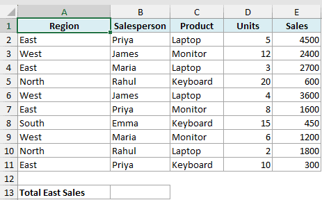
Here is the formula:
=SUMIFS(E2:E11,A2:A11,"East")
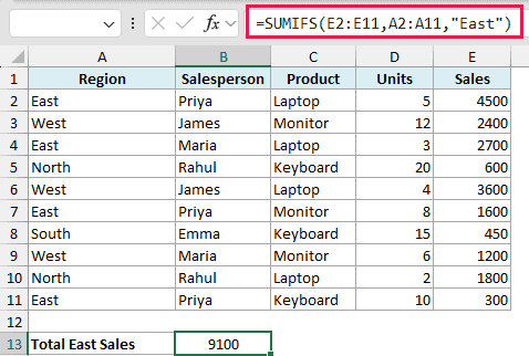
This gives me 9100.
Excel looks down the region column (A2:A11), finds every row that says East, and adds up the matching sales in column E. Everything that isn’t East is ignored.
Notice the text criteria “East” is wrapped in double quotes. Any text or logical condition you type directly into SUMIFS needs quotes around it.
Example 2: SUMIFS With Two or More Criteria
The real reason to reach for SUMIFS is checking more than one condition at once. Let’s add a second one.
I’m using the same sales table: region in column A, salesperson in column B, product in column C, units in column D, and sales in column E. This time I want the total sales for laptops sold in the East region.
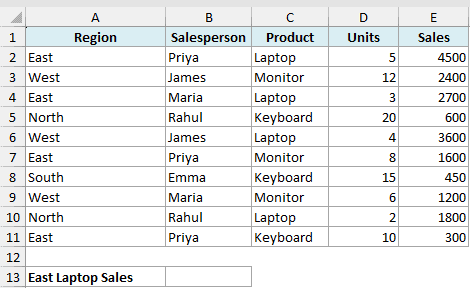
Here is the formula:
=SUMIFS(E2:E11,A2:A11,"East",C2:C11,"Laptop")
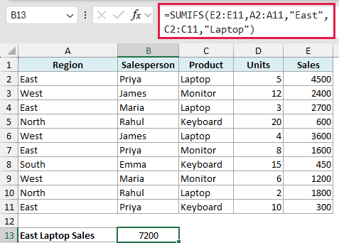
This returns 7200.
You just add another range and condition pair to the end. Now a row only counts if the region is East and the product is Laptop. Both have to be true.
You can keep stacking pairs like this. Want East laptops sold by a specific person? Add a third pair for the salesperson column. Every pair you add makes the condition stricter, since all of them must match.
Example 3: Using Comparison Operators in the Criteria
So far our conditions have been exact matches like “East”. But criteria can also be a comparison, like greater than or less than a number.
Here’s the same sales table, with units in column D and sales in column E. I want the total sales only for orders where more than 5 units were sold.
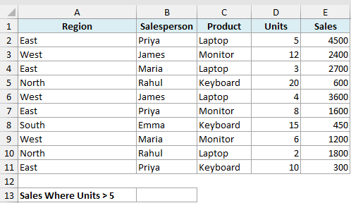
Here is the formula:
=SUMIFS(E2:E11,D2:D11,">5")
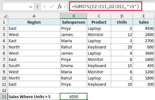
This gives me 6550.
The criteria “>5” tells Excel to only include rows where the units value is greater than 5. The comparison operator and the number both go inside one set of double quotes.
You can use any of the usual operators the same way: “>=100” for at least 100, “<50” for less than 50, or “<>0” for not equal to zero.
Follow along with the example file
SUMIFS Function Examples.xlsx
Example 4: Referencing a Cell in the Criteria
Typing conditions straight into the formula is fine, but it’s often better to point at a cell instead. That way you can change the condition without touching the formula.
Below the sales table I’ve set up a small criteria box: the region I want (East) sits in cell H2 and the minimum units value (5) in cell H3, each with a label beside it in column G. I want the total sales for that region where units are greater than or equal to that number.
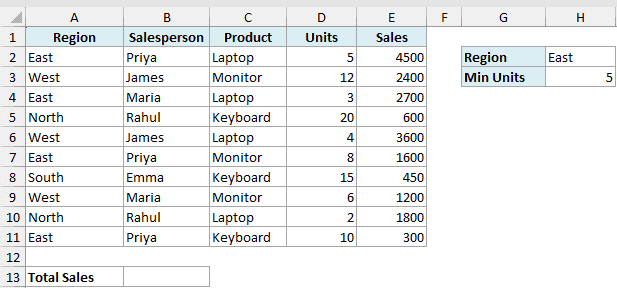
Here is the formula:
=SUMIFS(E2:E11,A2:A11,H2,D2:D11,">="&H3)
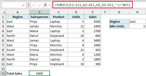
This returns 6400.
For the region, I just point at H2 directly, no quotes needed. For the units condition, I want “greater than or equal to whatever is in H3”, so I join the operator “>=” to the cell using the ampersand (&).
That & is the important bit. When you combine an operator with a cell reference, the operator stays in quotes and the cell reference stays outside, joined by &.
Now you can change East to West in H2, or 5 to 10 in H3, and the total updates on its own.
Example 5: Sum Between Two Dates
A very common use of SUMIFS is adding up amounts that fall between two dates. You do it with two conditions on the same date column: one for the start date and one for the end date.
Below I have an orders table with the order date in column A, the customer in column B, and the amount in column C. I want the total amount for orders placed between February 1, 2026 and March 31, 2026.
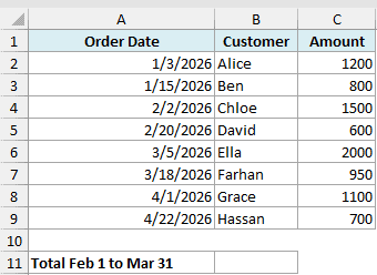
Here is the formula:
=SUMIFS(C2:C9,A2:A9,">="&DATE(2026,2,1),A2:A9,"<="&DATE(2026,3,31))
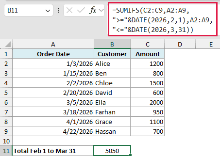
This gives me 5050.
The trick is checking the date column twice. The first pair keeps rows on or after the start date, and the second pair keeps rows on or before the end date. Together they leave only the rows inside the window.
I used the DATE function to build each date so Excel reads them correctly no matter your regional settings. If your start and end dates already sit in cells, you can point at those cells instead, like “>=”&F1 and “<=”&F2.
Example 6: Using Wildcards for Partial Matches
Sometimes you don’t want an exact match, just anything that contains or starts with certain text. That’s where wildcards come in. SUMIFS supports the asterisk (*) for any number of characters and the question mark (?) for a single character.
Here’s the same sales table, with the product in column C and sales in column E. I want the total sales for every product whose name starts with “Key” (so all the keyboards).
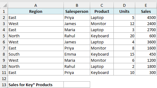
Here is the formula:
=SUMIFS(E2:E11,C2:C11,"Key*")
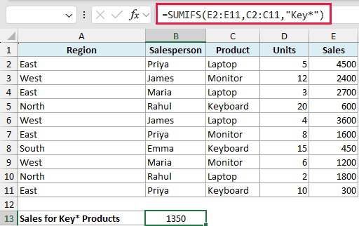
This returns 1350.
The asterisk after “Key” means “followed by anything”, so “Keyboard” matches. If you wanted products that merely contain a word, you’d wrap it in asterisks on both sides, like "*board*".
The question mark works the same way but for exactly one character. So “?ames” would match Names, James, or Games, but not Ames.
Pro Tip: If you need to match a literal asterisk or question mark (not use it as a wildcard), put a tilde (~) in front of it, like “~*” to find an actual asterisk.
Example 7: Get a Total per Category in One Formula (Dynamic Array)
Everything so far returns a single number in one cell, which is how SUMIFS is used most of the time. But if you’re on Microsoft 365, there’s a modern approach worth knowing.
Instead of writing a separate SUMIFS for each region, you can feed the list of unique regions into SUMIFS as the criteria and get one total per region, all from a single formula that spills down the sheet.
Here’s the same sales table, with the region in column A and sales in column E. I want a total for each region, listed out automatically.
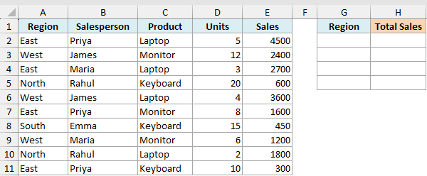
Here is the formula:
=SUMIFS(E2:E11,A2:A11,UNIQUE(A2:A11))
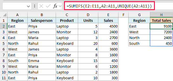
This spills a total for East, West, North, and South down the cells below.
Here is how it works:
- UNIQUE(A2:A11) pulls the list of distinct regions from column A (East, West, North, South).
- SUMIFS then runs once for each region in that list, so instead of one answer it returns a whole column of answers, one per region.
- Because you’re on 365, the results spill into the cells below automatically. You don’t drag anything down.
To see the region labels next to the totals, put =UNIQUE(A2:A11) in the column to the left. If you add a row below row 11, extend the ranges in both formulas to include it. Both spilled lists then update on their own.
Pro Tip: This spilling version needs Microsoft 365, Excel 2024, Excel 2021, or Excel for the web, since UNIQUE and spill ranges aren’t in Excel 2019 or earlier. On older versions, stick with one SUMIFS per category.
SUMIFS vs SUMIF: What’s the Difference?
Since the names are so close, these two get mixed up constantly. Here’s the clean split.
Use SUMIF when you have exactly one condition. Use SUMIFS when you have one condition or more. In other words, SUMIFS can do everything SUMIF does, plus handle multiple conditions.
The big gotcha is the argument order, which is reversed between them:
- SUMIF:
=SUMIF(range, criteria, [sum_range]), where the range you add comes last and is optional. - SUMIFS:
=SUMIFS(sum_range, criteria_range1, criteria1, ...), where the range you add comes first and is required.
Because SUMIFS covers the single-condition case too, a lot of people just use SUMIFS everywhere so they never have to remember two different argument orders.
Using SUMIFS in VBA
If you’re writing a macro, you can call SUMIFS through Excel’s WorksheetFunction object. The arguments go in the same order as the worksheet formula, with the sum range first.
Here is a small macro that sums the East region sales from our table and shows the answer in a message box:
Sub SumEastRegion()
    Dim total As Double
    total = Application.WorksheetFunction.SumIfs( _
        Range("E2:E11"), Range("A2:A11"), "East")
    MsgBox "Total East sales: " & total
End SubHere are the steps to use this macro:
- Press Alt + F11 to open the VBA editor.
- Insert a new module (Insert menu, then Module).
- Paste the code above.
- Press F5 to run it.
The WorksheetFunction.SumIfs call takes the ranges as Range objects and the criteria as text, just like the worksheet version. For a condition with an operator or a cell value, build the criteria as a string first, like ">=" & Range("H3").Value.
Tips and Common Mistakes to Keep in Mind
A few things that catch people out when they first use SUMIFS:
- Sum_range goes first. The most common mistake by far. In SUMIFS the range you add is the first argument, unlike SUMIF where it’s last.
- Keep every range the same size. The sum_range and all criteria_ranges must have the same number of rows, or you’ll get a #VALUE! error.
- Operators and text go in double quotes. Conditions like “>100”, “<>0”, or “East” all need quotes. Plain numbers and cell references don’t need quotes.
- Use & to join an operator with a cell. To compare against a value in a cell, write the operator in quotes and join it with &, like “>=”&H3. Don’t put the cell reference inside the quotes.
- SUMIFS uses AND, not OR. A row only counts when all your conditions are true. To add totals across “this OR that”, you’d sum two SUMIFS results together.
- Need to count instead of sum? The same multi-condition logic powers the COUNTIFS function, which counts rows that meet several criteria.
- SUMIFS ignores filters. It sums all matching rows even when some are filtered out of view. If you only want the visible rows, look at the SUBTOTAL function instead.
Wrapping Up
SUMIFS is one of those functions you’ll reach for constantly once it clicks. Start with a single condition, add more pairs as you need them, and lean on comparison operators, cell references, and wildcards to handle the trickier cases.
I hope you found this tutorial helpful. If you have a SUMIFS scenario you’re stuck on, it usually comes down to one of the common mistakes above.
Other Excel Articles You May Also Like:
