
There are many lookup functions in Excel (such as VLOOKUP, LOOKUP, INDEX/MATCH, XLOOKUP) that can go and fetch a value from a list.
But you can’t look-up images using these formulas.
For example. if I have a list of team names and their logos, and I want to look up the logo based on the name, I can’t do that using the inbuilt Excel function.
But that doesn’t mean it can’t be done.
In this tutorial, I will show you how to do a picture lookup in Excel.
It’s simple yet it’ll make you look like an Excel Magician (all you need is this tutorial and sleight of hands-on your keyboard).
Click here to download the example file.
Below is a video of the picture lookup technique (in case you prefer watching a video over reading).
Picture Lookup in Excel
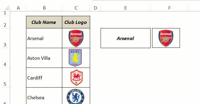
I have a list of the 20 teams in English Premier league (arranged in an alphabetical order) along with the club logo in the adjacent cell.

Now what I want is to be able to select a team name from the drop-down, and the logo of that selected team should appear.
Something as shown below:
There are four parts to creating this picture lookup in Excel:
- Getting the data set ready.
- Creating a drop-down list to show item names (club names in this example).
- Creating a Named Range
- Creating a Linked Picture.
Let’s go through these steps in detail now.
Getting the data ready
- Have the names of all the items (team names) in a column.
- In the adjacent column, insert the picture for the item (club logo in this example).
Make sure the logos fit nicely within the cell. You can resize the images so that these are within the cell, or you can expand the cells.
Creating the Drop-down list
- Select the cell in which you want the drop-down (E3 in this example).
- Click the Data tab.
- Click on the Data Validation option (it’s in the data tools category).

- In the Data Validation dialog box, within the Settings tab, make sure List is selected in the Allow drop-down (if not selected already).

- In the Source field, click on the upward-pointing arrow icon. This will allow you to select the cells in which you have the list for the dropdown.

- Select the range that has the club names (B3:B22 in this example).
- Hit Enter.
- Click OK.
The above steps would give you a drop-down list in cell E3.

Creating a Linked Picture
In this part, we create a linked picture using any of the existing images/logos.
Here are the steps to create a linked picture:
- Select any cell that has the logo. Make sure you have selected the cell, not the logo/image.
- Copy the cell (use Control + C or right-click and select copy).

- Right-click on the cell where you want to get the linked picture (it can be any cell as we can adjust this later).
- Go to the Paste Special option and click on the small right-pointing arrow to get more options.
- Click on the Paste Linked Picture icon.

The above steps would give you a linked picture of the cell that you copied. This means that if any changes happen in the cell that you copied, it will also be reflected in the linked picture).

In the above image, since I copied the cell C3 and pasted a linked picture. Note that this is not connected to the drop down as of now.
Also, when you paste the linked picture, it creates an image. So you can move it anywhere in the worksheet.
Creating a Named Range
Now we have everything in place, and the last step is to make sure that the linked picture updates when the selection is changed. As of now, the linked picture is linked to only one cell.
We can connect it to the drop-down selection by using a named range.
Here are the steps to do this:
- Go to the Formulas tab.
- Click on the Define Name option. This will open the ‘New Name’ dialog box.

- In the New Name dialog box, make the following entries:
- Name: ClubLogoLookup
- Refers to: =INDEX($C$3:$C$22,MATCH($E$3,$B$3:$B$22,0))

- Click OK.
- Select the linked image that we created in the previous step. You will notice a cell reference in the formula bar (for example =$C$3). Delete this cell reference and type =ClubLogoLookup.

That’s it!! Change the club name from the drop-down and it will change the picture accordingly.
How does this Picture Lookup Technique work?
When we created a linked picture, it was referring to the original cell from which it was copied. We changed that reference with the named range.
This named range is dependent on the drop-down and when we change the selection in the drop-down, it returns the reference of the cell next to the selected team’s name. For example, if I select Arsenal, it returns, C3 and when I select Chelsea, it returns C6.
Since we have assigned the named range to the linked picture (by changing the reference to =ClubLogoLookup), it now refers to the new cell references, and hence returns an image of that cell.
For this trick to work, the defined name should return a cell reference only. This is achieved by using the combination of INDEX and MATCH functions.
Here is the formula:
=INDEX($C$3:$C$22,MATCH($E$3,$B$3:$B$22,0)).
The MATCH part in the formula returns the position of the club name in the drop-down. For example, if it’s Arsenal, MATCH formula would return 1, if its Chelsea then 4. The INDEX function locates the cell reference that has the logo (based on the position returned by MATCH).
Try it yourself.. Download the Example file from here

You May Also Like the Following Excel Tutorials:


This helped me a lot on my mini project! search from another instruction but not working, this Index & Match works pretty well Thanks 🙂
I found this solution on a different website (that I can’t find now), but I got it working and it’s great. However, I want to have lots of picture cells referencing the same table of pictures, but independently sourced. For example, using the table in the tutorial, I’d like to have more drop down menu cells that can display different pictures in the adjacent picture. I can do it, but I have to create a new “Define Name” reference on the “Name Manager” for each new picture I want to create. The problem is, the more names that are defined, the slower Excel becomes. Is there a way to do that without having to define a new name for each picture reference cell? Or is there a different way to do this where Excel doesn’t slow down?
tried all the above solutions, but still giving error “reference is not valid”
I am unable to change the cell reference to named range. Gives error “reference is not valid”. I am unable to fix this. Any guidance as to what could be reason for this error?
Could you solve the problem? Its happening to me too..
THANK YOU! I have been trying to find a way to do an image lookup all day, and between your video and written instructions, I finally got this to work. You made my day!!!
This solved one issue I had; really well explained and modified easily – thank you very much for that!
It did raise another issue, though: I’d like to pull the cell that shows the image into a generated PDF. I’m using VBA and pulling different cell ranges from different worksheets together. That part works fine.
But the variable image in your example isn’t actually part of the cell; it’s locked to it, but it “floats” above the cell while the cell is blank, meaning my script is just pulling the blank content of the cell.
Do you know of a way to incorporate the (variable) image into the cell content directly/embed it?
Amazing! This is fantastic. I have noticed it seems to affect performance a bit. Is there any way to avoid that? I feel like excel responsiveness deteriorates once this is put in place.
Hi Sumit,
I did all the steps and when I look up I get a zero instead of the picture
hi,
i have a table of 250 cells in one column and 15 column in one rwo i want to insert symbols in saperate column max 4 symbol one in each column based on value in refrence cell in same row can you please help
Is there a way for this to work with a Filter from a Pivot Table. For example, when I filter by Name on my Pivot table, can I get the picture changed instead of doing the List Box in the cell to the left?
I made a picture vlookup according this formula, but I am not getting sharp image why ?
I agree with the other commenters that this works better than any of the other step-by-step guides I have found for this. However, I am having trouble duplicating the process beyond the first dropdown/photo cell. What is the process for repeating this for the rest of the worksheet? Thanks!
I have done as above instruct but it still show reference is not valid
You must type “Arsenal” or any name of club in cells E3 before do:
Step 5. Select the linked image that we created in the previous step. You will notice a cell reference in the formula bar (for example =$C$3). Delete this cell reference and type =ClubLogoLookup.
NOT WORKING, STILL SHOWING ERROR “REFERENCE IS NOT VALID”, PL HELP
My problem solved: lock all cell references in formula before copying to name manager.
Thank you for a very easy, uncomplicated and great explanation. The previous examples I tried from other websites were complicated, confusing and did not work.
hi Sumit,
i have one concern ,i am trying to do image lookup in one excel file to another excel,but it was not coming .so kindly need your help on this.
Hi Sumit.
I have an issue when i try to link the formula to the image. When i type = and the name of the formula i have given im getting this message: Reference is not valid.
Can you please help me understand my error?
Hi. I had the same problem. My excel was in Spanish, so once I wrote the formulas in Spanish, the error dissapeared.
You must type “Arsenal” or any name of club in cells E3 before do:
Step 5. Select the linked image that we created in the previous step. You will notice a cell reference in the formula bar (for example =$C$3). Delete this cell reference and type =ClubLogoLookup.
What if I don’t want the drop down list. Instead of new list?
Sumit,
How can I do if I have two drop down lists? I want to show the image if one of the list change. I’m practicing a musical instrument and I wanted to show the image, in example, Cmaj,Cmin,Cdim; one combo is made by principal notes: C,Cb,D,Db… and the other list is the chord: Major, minor, aug, dim, sus, 6…
Thanks in advance
Thank you so much with this. I was wrecking my head with macos that didn’t always work. This was so much easier to do.
Hi, can it be done in userform?
Thank you so much.It was awesome.
Hi I tried but it keeps popping out “The reference is not valid”. I tried with exact same format like yours but still not working
You must type “Arsenal” or any name of club in cells E3 before do:
Step 5. Select the linked image that we created in the previous step. You will notice a cell reference in the formula bar (for example =$C$3). Delete this cell reference and type =ClubLogoLookup.
Hey this works in excel 2010?
Yes it does, I just did it in Excel 2010.
Hey, Thanks for Sharing, i just have a question, i merged couple of cells and pasted the picture in and sized as the merged cell, the problem is whenever i close and re open the file, the picture comes small again.
Can you help with that, thank you 🙂
I’ve done something similar before using images on points in a scatterplot and some vba code to pick the right axis scales from a lookup list to show each picture…but this is a thousand times simpler. Now have a series of maps dynamically changing in my workbook (and linked to a powerpoint document too) – awesome!
Thanks for commenting Andy.. Glad you found it useful 🙂
Hello,
I have a question. In this example the filter cell is E3 and the image is in G3.When i chose a team the image is changing.
I want to do this filter in all th cell E:E.If i choose a team in E4 it changes the images in G4, if i choose a team in E5 it changes the imagine in E58,etc.
Thank you very much.
Hello Bogdan.. Welcome to Trump Excel!
Yes this can be done. You will have to create multiple named ranges (ClubLogoLookup2, ClubLogoLookup3, and so on..). Just change the reference from $E$3 to $E$4 and so on.
Here is a sample file – http://goo.gl/Cwk6ls
Hello Sumit… I tried to see your sample files ( http://goo.gl/Cwk6ls) but they were moved out. On another note, How could you use your technique if “Club Names and Logos” and “Validation Drop Down and Cell showing Selected Club Logo” are in a different workbooks?
Your help is really appreciated…
Hello, This is a great trick. However, when I try to try to create the dynamic image in a different tab it never works. Is there a specific trick that I have to do?
You have to name the two tabs you’re using in the formula. Be specific about which tab has the images and which tab you want the dynamic image to be in as well as which column has the words that are tied to the individual pictures.
Something like this:
=INDEX(‘Tab1’!$J$7:$J$30,MATCH(‘Tab2′!$A$13,’Tab1’!$D$7:$D$30,0))
Thanks a lot Dave. That helps so much. I was finally able to do it. Much appreciated.
Is there a limit to how many cells this formula extends to? I’m using this formula because another similar one I used stopped retrieving pictures at row 2727. Does this formula have that same problem?
THANK U VERY MUCH.THE TIP VERY USEFUL TO ME
Thanks Sampath.. Glad it helped 🙂
Thank you! This helps a lot! Are you able to move the dropdown bar to a different tab? Instead of having next to the pictures?
Thanks Carla.. This techniques works even if you move the drop down to some other tab