Combine CSV Files When Column Headers Don’t Match

When you combine multiple CSV files using Power Query, it works great if all files have the same column names.

But what if they don’t? What if one file calls it “Sales Rep” and another calls it “Salesperson”? One says “Units Sold” and another says “Quantity Sold”?

Power Query treats these as separate columns, leaving you with a messy table full of null values.

In this article, I’ll show you how to fix this using a mapping table in Power Query. It takes some setup, but once it’s in place, it handles any combination of inconsistent headers automatically.

Download Example File | Files Used in this Example (ZIP Folder)

The Problem: null Values from Mismatched Headers

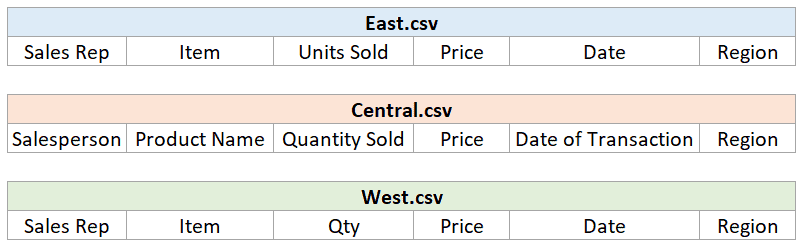
Let’s say you have three CSV files: East, Central, and West.

They all contain the same sales data, but the column names aren’t consistent.

For example, East.csv has a column called “Sales Rep” while Central.csv calls the same column “Salesperson.”

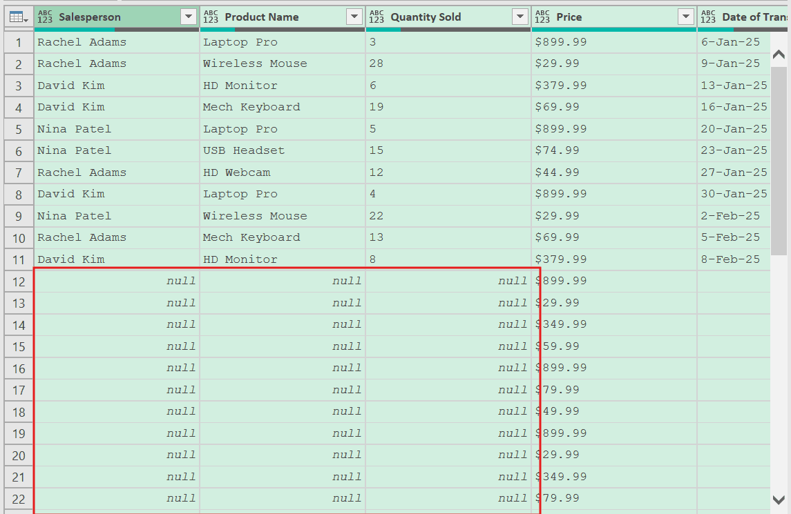
When you combine these files using the standard Power Query approach, here’s what happens:

Power Query doesn’t know “Sales Rep” and “Salesperson” are the same column. So it creates two separate columns for both. The result is partial data in each column, with a lot of null values filling in the gaps.

The fix – using a mapping table.

You create a mapping table to tell Power Query which column names represent the same data, so it can standardize them before combining everything.

The 3-Step Approach

Here’s a quick overview before we get into the details:

1. Extract all column names from all your CSV files and load them into Excel
2. Create a mapping table by manually assigning a standardized name to each column header
3. Combine the CSV files using the mapping table to rename columns before merging

Step 2 is the only manual step, and you only need to do it once.

Step 1: Extract All Column Names from Your CSV Files

The goal here is to get a complete list of every column name used across all your CSV files, including all the inconsistent variations.

Connect Power Query to the Folder with CSV Files

1. Go to the Data tab
2. Click Get Data > From File > From Folder

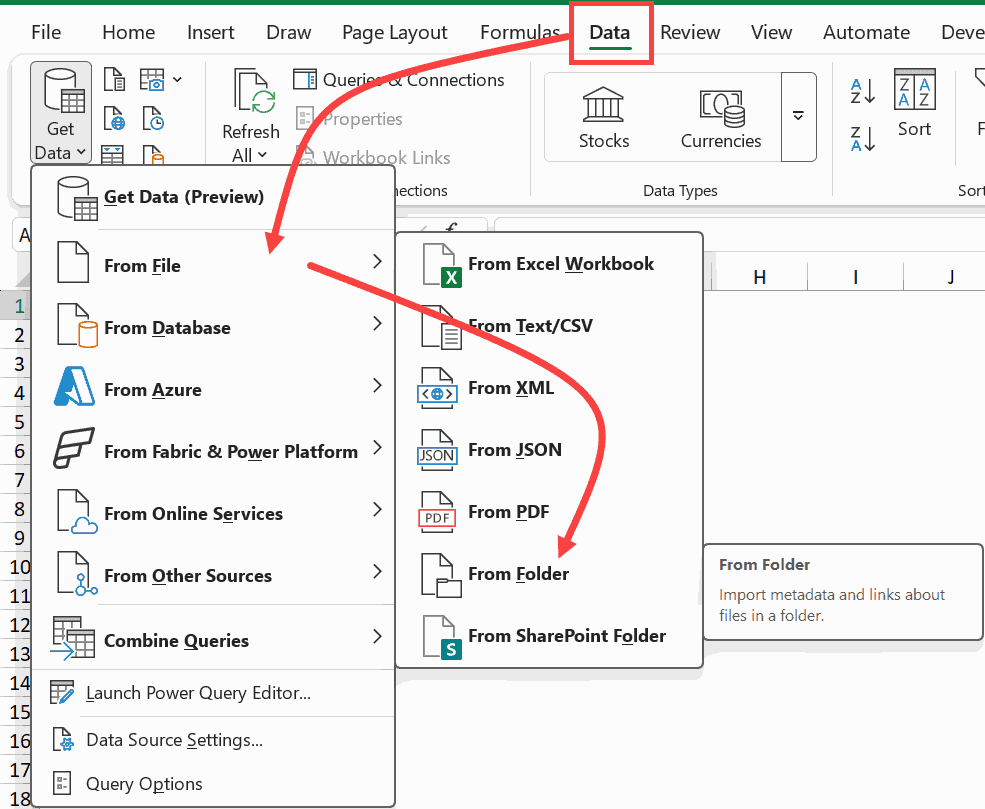
3. Browse to the folder that contains your CSV files and click Open
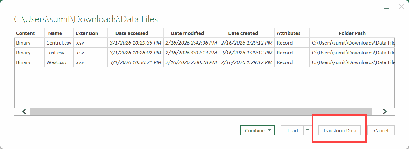
4. Power Query shows all the files in the folder. Click Transform Data to open the Power Query Editor

Filter for CSV Files Only

This is an important step to future-proof your query. If someone later adds files other than the CSV files (such as PDF, Excel, or text files), your query won’t break.

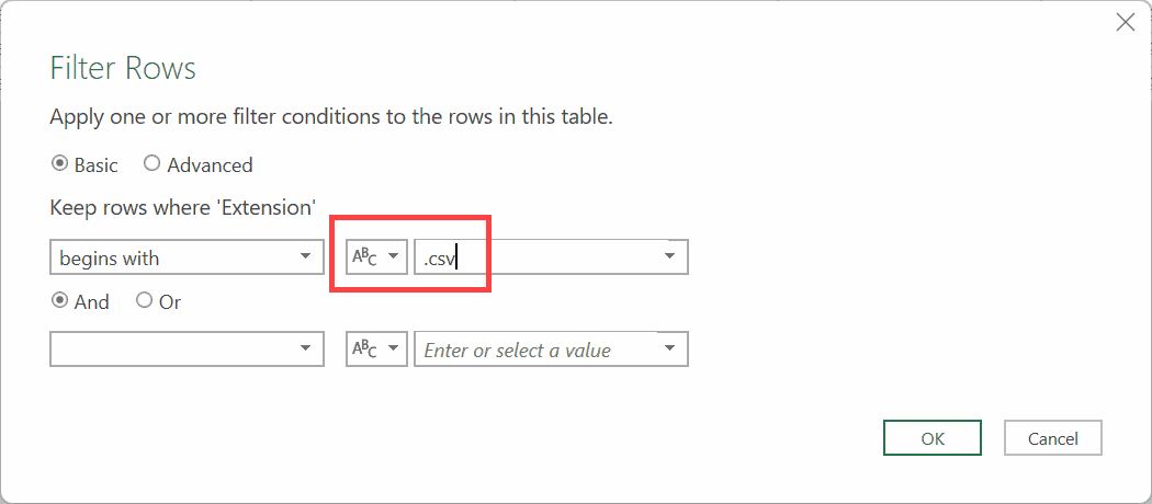
5. Click the dropdown arrow on the Extension column
6. Go to Text Filters > Begins With

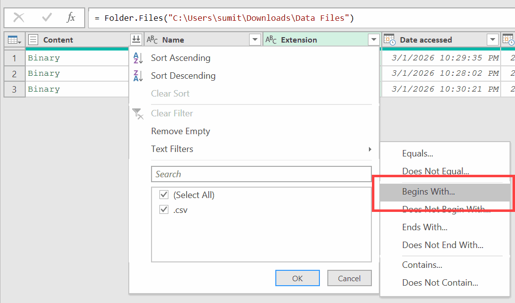
5. Type .csv and click OK

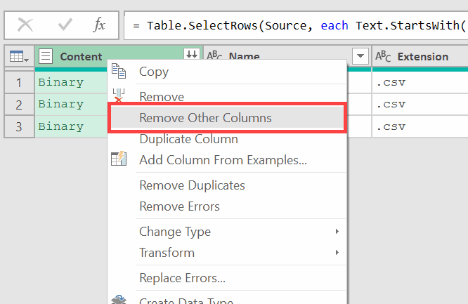
Keep only the Content column

8. Right-click the Content column (the binary column that holds the file data) and select Remove Other Columns

Extract the Table from Each CSV File

9. Go to the Add Column tab and click Custom Column

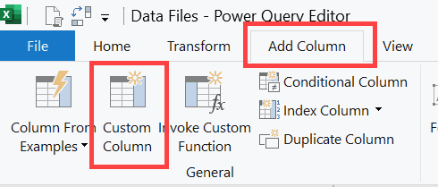
10. Name the column Custom
11. Enter this formula:

Table.PromoteHeaders(Csv.Document([Content]))

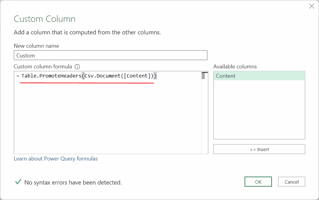
In the above formula, Csv.Document([Content]) reads each binary file and returns the data in that file as a table in this newly added column.

Table.PromoteHeaders() then promotes the first row to column headers in all the tables.

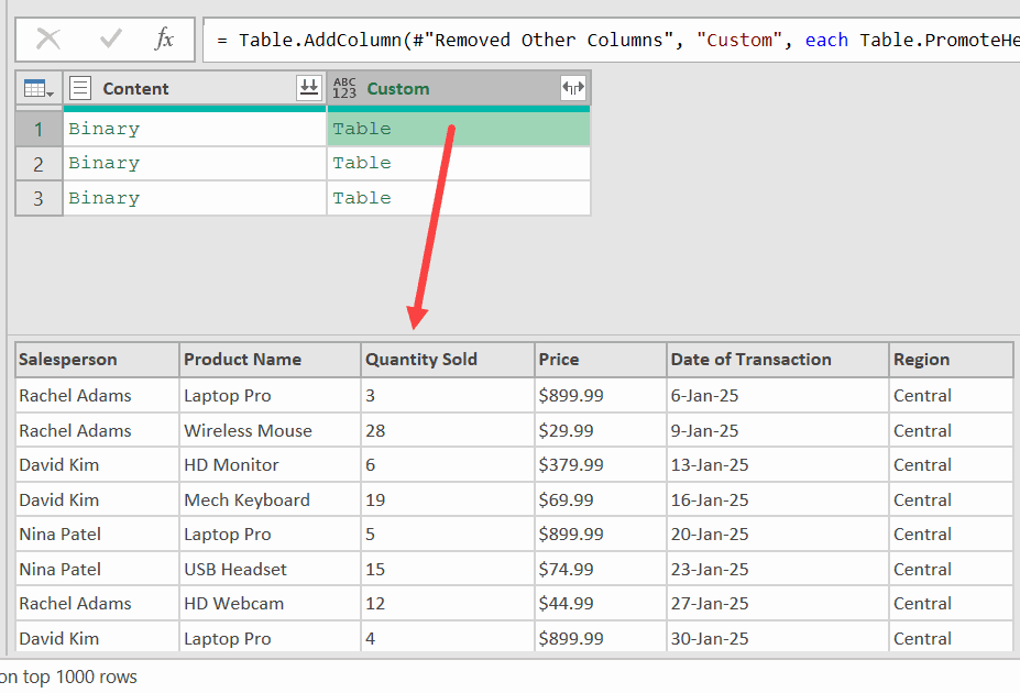
12. Click OK

You’ll see a “Table” value in each row. Click on any of them, and the preview at the bottom shows the data for that file, including its specific column headers.

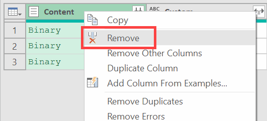
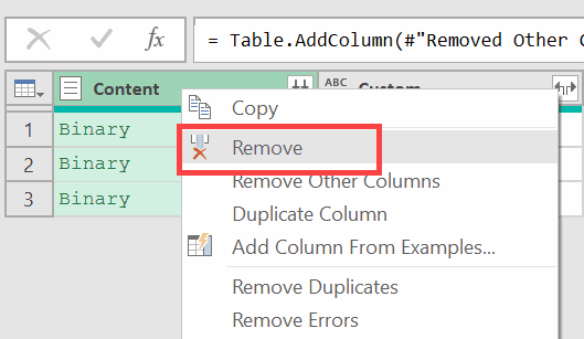
Combine All Tables and Extract the Column Names:

13. Right-click the Content column and select Remove

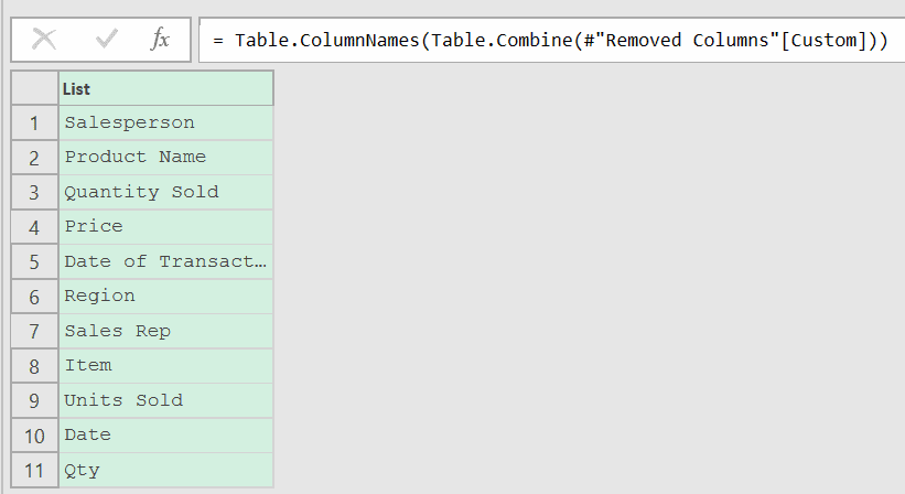
14. In the formula bar, click fx to add a new step. Enter:

= Table.ColumnNames(Table.Combine(#"Removed Columns"[Custom]))

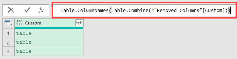
Here’s what this formula does:

• “Removed Columns”[Custom] gets the list of tables from the Custom column
• Table.Combine(…) stacks all the tables into one (you’ll see nulls from the mismatched headers, but that doesn’t matter here)
• Table.ColumnNames(…) pulls out every column name from the combined table

You now have a list of all column names from every CSV file, including all the inconsistent variations.

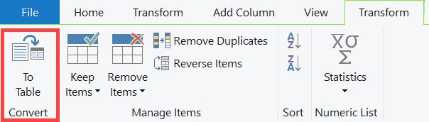
Load the Column Names to Excel

15. Click To Table in the List Tools tab and click OK to convert the list to a table

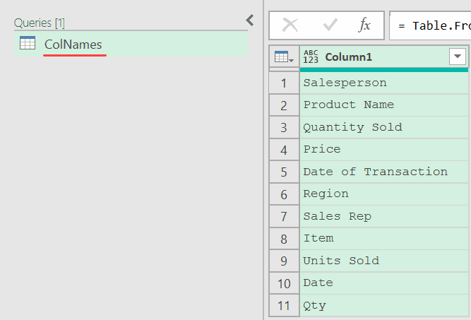
16. In the Query Settings pane on the right, rename the query to ColNames

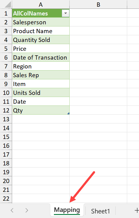
17. Rename the column name to AllColNames

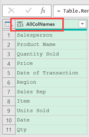
16. Click Close & Load

Excel creates a new sheet with all your column names in one column. Rename this sheet Mapping so it’s easy to find later.

Step 2: Create the Mapping Table

Now you have every column name from every CSV file sitting in your Excel sheet.

Time to set up the mapping.

Add a new column next to the existing one. Call it New Names.

For each row, type the standardized column name you want to use in the final combined table. Here’s what this looks like:

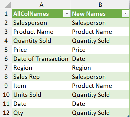
The logic is simple. If two column names contain the same data, give them the same New Name.

Power Query uses this table to standardize all column names before combining the files.

If a column name is already what you want (like “Price” or “Region”), just repeat it in the New Names column.

This is a one-time setup.

In the future, when new files arrive with new column names, you’ll see blank rows in the New Names column after a refresh. Just fill those in, and you’re good to go.

Step 3: Combine the CSV Files Using the Mapping Table

This step has two parts: loading the mapping table into Power Query as a reference, then using it to combine all the CSV files cleanly.

Part 1: Load the Mapping Table into Power Query

1. Click anywhere inside the mapping table in your Excel sheet
2. Right-click and select Get Data from Table/Range

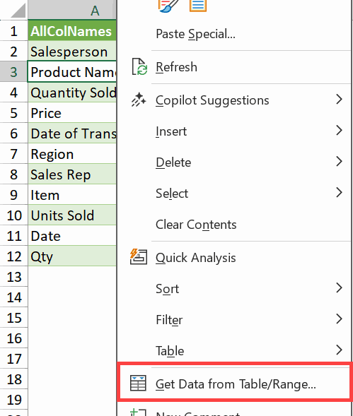
3. Power Query opens with your mapping data
4. In the Query Settings pane, rename the query MappingTable (no spaces make it easier to reference in formulas)
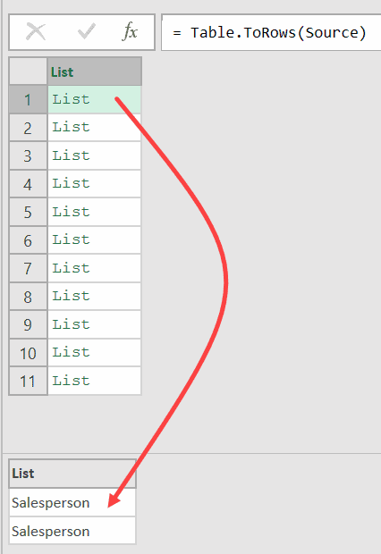
5. Click fx in the formula bar to add a new step. Enter:

= Table.ToRows(Source)

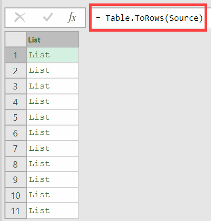
This converts each row into a two-item list like {“Sales Rep”, “Salesperson”}. That’s the exact format Table.RenameColumns expects.

6. Go to File > Close & Load To
7. Select Only Create Connection and click OK

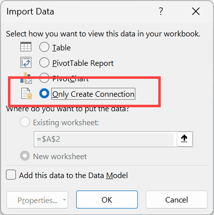
The mapping table is now available as a reference inside Power Query.

Part 2: Connect to the CSV folder and combine the files

8. Go to Data > Get Data > From File > From Folder
9. Select the same folder with CSV files and click Open
10. Click Transform Data

Do the same setup as Step 1:

11. Filter the Extension column: Text Filters > Begins With > .csv
12. Right-click the Content column and select Remove Other Columns

Add the custom column with renaming:

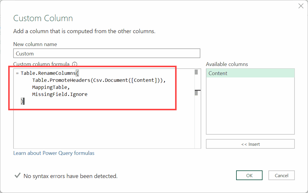
13. Go to Add Column > Custom Column
14. Name the column Custom and enter this formula:

Table.RenameColumns(
    Table.PromoteHeaders(Csv.Document([Content])),
    MappingTable,
    MissingField.Ignore
)

Here’s what each part does:

• Csv.Document([Content]) reads the binary file as a CSV
• Table.PromoteHeaders(…) promotes the first row as column headers
• Table.RenameColumns(…, MappingTable, MissingField.Ignore) renames the columns using your mapping table. MissingField.Ignore tells Power Query to skip any rename pair where the column doesn’t exist in that particular file.

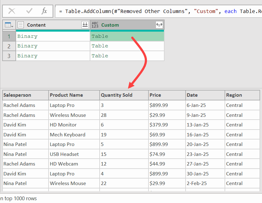
15. Click OK

Click on any of the table values in the Custom column. The column headers are now consistent across all files.

Combine all tables:

16. Right-click the Content column and select Remove

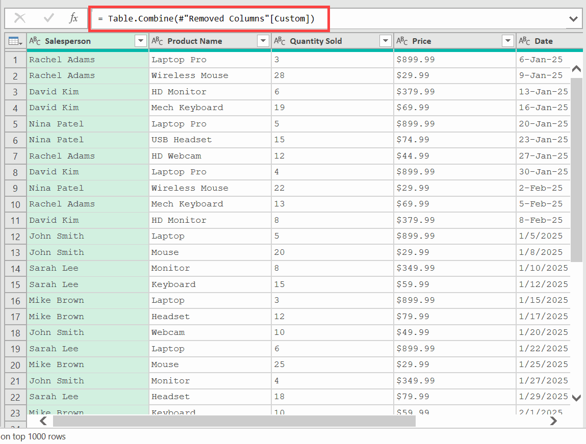
17. In the formula bar, click fx to add a new step. Enter:

= Table.Combine(#"Removed Columns"[Custom])

Your data is now combined with consistent column names throughout.

18. Click Close & Load To and choose where you want the data in Excel

Done. No null values, no mismatched columns.

What Happens When You Add New Files

Here’s where the one-time setup pays off.

If you drop a new CSV file into the folder and it has a column name you haven’t mapped yet:

1. Right-click the mapping table in Excel and click Refresh
2. Any new column names will appear with blank New Names cells
3. Fill in the standardized name for each new row
4. Right-click your combined data table and click Refresh

The query picks up the new file, applies the updated mapping, and adds the new rows to the combined table automatically.

Don’t try to refresh the combined query before filling in the blanks, else you’ll get an error. Power Query needs a valid rename pair for every row in the mapping table, and blank New Names cells will cause it to fail.

Tips & Common Mistakes

• Always filter for .csv files. Without this filter, any non-CSV file that ends up in the folder will break your query. It takes about 20 seconds to set up and saves a lot of headaches later.
• Don’t skip MissingField.Ignore. Not every column exists in every file, and without this argument, Power Query throws an error the moment it tries to rename a column that isn’t there.
• Column names are case-sensitive in Power Query. “Salesperson” and “salesperson” are treated as different columns. Make sure your mapping table accounts for every variation, including capitalization differences.
• Load the mapping table as connection-only. You already have the mapping data visible in your Excel sheet. If you also load the Power Query result as a table, you’ll end up with duplicate data in your workbook.
• Fill in every blank in the New Names column before refreshing. A single empty cell causes an error. Every old column name needs a corresponding new name.

The setup takes some effort the first time.

After that, adding new files is just a refresh and filling in any new column names that show up.

In this article, I showed you how to combine all the CSV files in a folder when the column header names are inconsistent.

I hope you found this article helpful.

Other Excel & Power Perry articles you may also like:

• Combine Data from Multiple Workbooks in Excel (using Power Query)
• Get a List of File Names from Folders & Sub-folders (using Power Query).
• Merge Tables in Excel Using Power Query
• How to Combine Multiple Excel Files into One Excel Workbook.
• Combine Data From Multiple Worksheets into a Single Worksheet in Excel.
• Split Each Excel Sheet Into Separate Files
• Get Today’s Date in Power Query