

If you want to look up a value across a row and pull back a matching value from a row below it, the HLOOKUP function is what you need.
It searches the top row of a table from left to right, and once it finds your value, it drops down to grab an answer from a row you point it to.
Most people reach for VLOOKUP, which works down a column. HLOOKUP is the same idea turned sideways, and it’s the right pick when your labels run across a row instead of down a column.
In this article, I’ll show you how to use HLOOKUP with real examples, how to pair it with MATCH for a flexible row number, and how the newer XLOOKUP function handles the same job in Excel 365 and 2021.
Follow along with the example file
HLOOKUP Function Examples.xlsx
When to Use the HLOOKUP Function
HLOOKUP is built for horizontal data. If your headings sit across the top row (months, regions, quarters) and the values you want are stacked in rows below those headings, HLOOKUP is the fit.
You give it a value to find in the top row. When it finds a match, it moves straight down that column and returns whatever sits in the row number you asked for.
The one thing to remember: HLOOKUP only looks down from the top row. It can’t look up. So the row you’re searching has to be above the row you want the answer from.
HLOOKUP Syntax and Arguments
Here is the syntax of the HLOOKUP function:
=HLOOKUP(lookup_value, table_array, row_index_num, [range_lookup])
- lookup_value – the value you want to find in the top row of the table. This can be a number, text, or a cell reference.
- table_array – the range that holds your data, including the top row where the lookup happens and every row you might pull an answer from.
- row_index_num – the row number in the table that holds the value you want back. Row 1 is the top row itself, row 2 is the row right below it, and so on.
- range_lookup – optional. Use FALSE for an exact match, or TRUE (the default) for an approximate match. More on this below.
Pro Tip: When range_lookup is left out, HLOOKUP assumes TRUE and looks for an approximate match. That surprises a lot of people, so type FALSE whenever you want an exact match.
Example 1: HLOOKUP Exact Match Example
Let’s start with the most common use. Below is a small sales table where the region names sit across the top row and the sales and manager rows are stacked below them. I want to find the Q2 Sales figure for the East region.
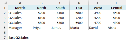
Here HLOOKUP searches the top row for “East”, then drops down to row 3 (the Q2 Sales row) and returns that value. Here is the formula:
=HLOOKUP("East",A1:F5,3,FALSE)
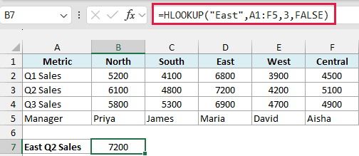
This returns 7200, which is the Q2 Sales figure sitting in the East column.
The FALSE at the end forces an exact match, so HLOOKUP returns a value only when it finds “East” spelled exactly. Row 3 is counted from the top of the table range, so row 1 is the header row, row 2 is Q1 Sales, and row 3 is Q2 Sales.
Example 2: HLOOKUP with MATCH for a Dynamic Row Number
Now let’s make the formula smarter. Typing 3 for the row number works, but if you add or move rows, that hard number breaks. MATCH can find the right row number for you, so the formula keeps working.
Below is the same sales table. This time I want the Q3 Sales figure for the West region, without counting rows by hand.
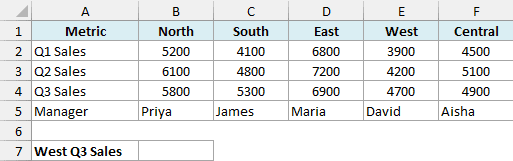
MATCH looks for “Q3 Sales” down the first column and returns its position, which HLOOKUP then uses as the row number. Here is the formula:
=HLOOKUP("West",A1:F5,MATCH("Q3 Sales",A1:A5,0),FALSE)
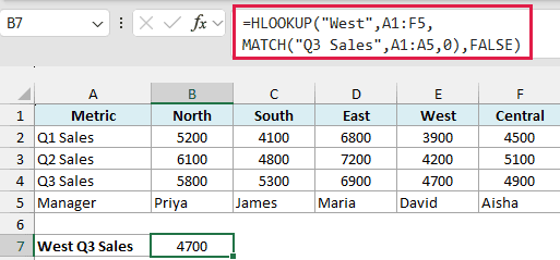
This returns 4700, the Q3 Sales value in the West column.
Here MATCH(“Q3 Sales”,A1:A5,0) looks down A1:A5 and finds “Q3 Sales” in the fourth position, so it hands the number 4 to HLOOKUP. Because MATCH does the counting, you can rearrange or insert rows and the formula still points at the right one.
Example 3: HLOOKUP Approximate Match Example
HLOOKUP can also find the closest match instead of an exact one. This is handy for lookups like tax brackets or commission tiers, where a value falls into a range rather than matching a single number.
Below is a commission table. The sales thresholds in B1:E1 run in ascending order, and the matching rates sit below them. I want the rate that applies to sales of 7500, so the lookup range excludes the labels in column A.
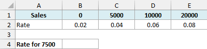
With TRUE as the last argument, HLOOKUP looks for the largest value that is still less than or equal to 7500. Here is the formula:
=HLOOKUP(7500,B1:E2,2,TRUE)
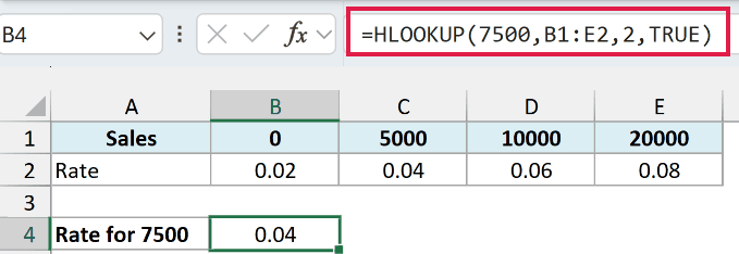
This returns 0.04 (a 4% rate). There’s no 7500 in the top row, so HLOOKUP settles on 5000, the largest threshold that doesn’t go over 7500, and returns the rate below it.
Pro Tip: For an approximate match to work, the top row must be sorted in ascending order from left to right. If it isn’t sorted, HLOOKUP can return the wrong value.
Example 4: Use XLOOKUP for Horizontal Lookups (Modern Alternative)
If you’re on Excel 365 or Excel 2021, XLOOKUP is the cleaner way to do the same lookup. It works horizontally too, you don’t have to count row numbers, and it does an exact match by default.
Below is the sales table again. I want the same answer as the first example, the Q2 Sales figure for the East region.
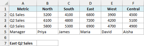
Instead of a row number, you hand XLOOKUP the row to search and the row to return from. Here is the formula:
=XLOOKUP("East",B1:F1,B3:F3)
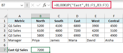
This returns 7200, the same East Q2 Sales value HLOOKUP gave us earlier.
XLOOKUP searches the region names in B1:F1, finds “East”, and returns the value in the matching position of B3:F3 (the Q2 Sales row). It matches exactly by default, so there’s no FALSE to remember, and it isn’t tied to a fixed row_index_num.
Pro Tip: XLOOKUP is only in Excel 365, Excel 2021, and later. On Excel 2019 or 2016, stick with HLOOKUP or the HLOOKUP with MATCH combo shown above.
Tips and Common Mistakes
A few things trip people up with HLOOKUP, so keep these in mind:
- It only looks down, never up. HLOOKUP searches the top row and returns from a row below it. If the row you want sits above your search row, HLOOKUP can’t reach it. XLOOKUP or an INDEX and MATCH combination can look in any direction.
- Forgetting FALSE can give you the wrong answer. Leave range_lookup out and HLOOKUP runs an approximate match. It may return a value or #N/A, so add FALSE whenever you need an exact match.
- A #N/A error can mean no exact match was found. With approximate matching, it also occurs when your lookup value is smaller than the first threshold. For exact matches, check for extra spaces, a typo, or numbers stored as text.
- A #REF! error means row_index_num is too big. If you ask for row 6 in a table that’s only 5 rows tall, HLOOKUP returns #REF!. Make sure the row number fits inside your table range.
- Approximate match needs a sorted top row. With TRUE, sort the top row in ascending order from left to right, or the result can be off.
Wrapping Up
HLOOKUP is the horizontal cousin of Excel’s VLOOKUP function, and it’s the right tool when your data runs across a row instead of down a column.
Pair it with MATCH when you want a flexible row number, and switch to XLOOKUP when you’re on a version that has it, since it looks in any direction without the row counting.
I hope you found this tutorial helpful. Let me know in the comments if you have any questions.
Other Excel Articles You May Also Like:
