

You wrote a VLOOKUP, hit Enter, and instead of the value you expected you got a #N/A error (or worse, a wrong number).
It’s one of the most frustrating things in Excel, and it almost always comes down to a small mismatch between what you’re looking up and what’s actually sitting in your table.
The good news is that VLOOKUP fails for a handful of predictable reasons, and each one has a quick fix. In this article I’ll walk through the 10 most common reasons your VLOOKUP isn’t working, with a fix for each.
The Sample Data I’ll Use
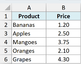
For most of the examples I’ll use this little price list. Column A has the product and column B has the price, and I want to look up a price by the product name.
A few of the fixes need a different layout to show the problem, so I’ll set those up as we go. Let’s start with the reason I see most often.
1. You’re Using Approximate Match by Leaving Out the Last Argument
VLOOKUP’s fourth argument decides whether you get an exact match or an approximate one. Leave it out, and Excel defaults to approximate match, which is almost never what you want for names and text.
Here’s the formula with the last argument missing:
=VLOOKUP("Apples",A2:B6,2)
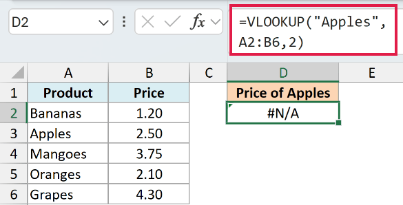
Apples is sitting right there in A3, but the formula returns #N/A. Approximate match assumes the first column is sorted, and this one isn’t, so VLOOKUP gives up before it gets there.
Sometimes it’s worse than an error. Look up Grapes the same way and you get 2.50 back, which is the price of Apples, with nothing to tell you it’s wrong.
The fix is to add FALSE (or 0) as the fourth argument, which forces an exact match:
=VLOOKUP("Apples",A2:B6,2,FALSE)
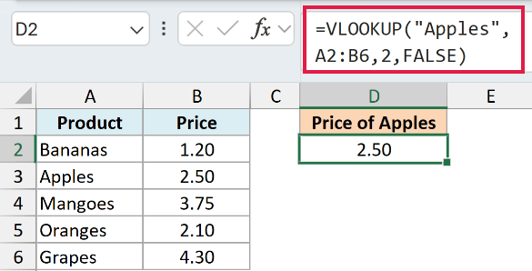
Now it returns 2.50, the correct price. Get into the habit of always adding FALSE unless you specifically need a range lookup.
2. The Lookup Value Isn’t in the First Column of the Table
VLOOKUP only ever searches the first column of the table you hand it. If the value you’re looking up lives in a column to the right of your answer, VLOOKUP simply can’t see it, because it doesn’t look left.
Say I have an employee list with names in column A and IDs in column B, and I want to find a name from an ID. The obvious formula looks like this:
=VLOOKUP(105,A2:B6,1,FALSE)
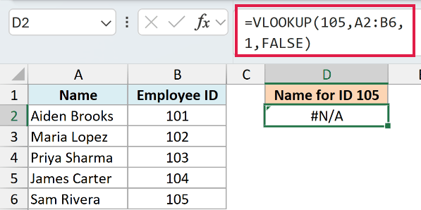
#N/A, even though ID 105 is clearly in the list. VLOOKUP searched column A for 105, found nothing but names there, and gave up. It never looked at column B at all.
The cleanest fix is to switch to INDEX MATCH, which can look in any direction:
=INDEX(A2:A6,MATCH(105,B2:B6,0))
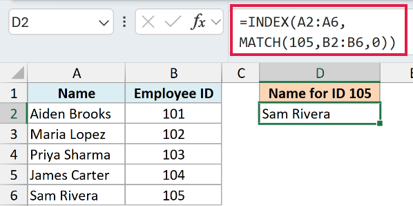
This finds ID 105 in column B and returns the name from column A, “Sam Rivera”. If you’d rather learn the pairing properly, here’s the full INDEX MATCH combo.
XLOOKUP handles left lookups too, if you’re on Excel 365 or 2021.
3. Extra Spaces or Non-Printing Characters
This one is sneaky because everything looks correct on screen. If the cell you’re looking up says “Apples ” with a trailing space, it won’t match the “Apples” in your table, and you’ll get a #N/A.
Extra spaces usually creep in from copy-pasting or exports from other systems. Non-printing characters do the same thing, and you can’t even see them.
=VLOOKUP(D2,A2:B6,2,FALSE)
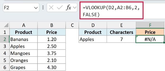
The lookup value in D2 reads Apples and the table has Apples, but the result is #N/A. I’ve put a character count next to it, and that’s the tell: LEN says 7 characters for a 6-letter word. There’s a space on the end you can’t see.
TRIM removes extra spaces and CLEAN strips out non-printing characters. If the stray spaces are in your lookup value, you can wrap it like this:
=VLOOKUP(TRIM(D2),A2:B6,2,FALSE)
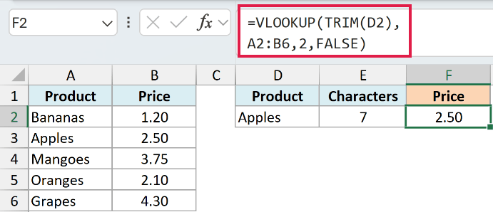
Same data, same character count, but now it returns 2.50.
If the spaces are in the table itself, TRIM on the lookup value won’t help. In that case, clean the source data directly, either with Find and Replace or a helper column of =TRIM(CLEAN(A2)) that you paste back over the originals as values.
4. Numbers Stored as Text (or the Other Way Around)
To Excel, the number 101 and the text “101” are two different things. If your table stores employee IDs as real numbers but the ID you’re looking up is stored as text (or vice versa), VLOOKUP won’t find a match.
=VLOOKUP(D2,A2:B6,2,FALSE)
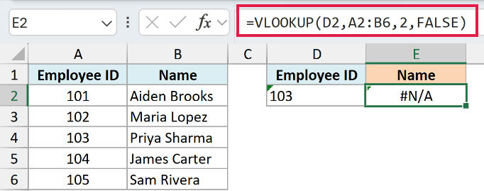
ID 103 is right there in the table, but the lookup value is text and the table holds real numbers, so they never match.
The tell-tale signs are in the picture. The 103 I’m looking up hugs the left edge of its cell while the IDs in column A sit centered, and there’s a little green triangle in the corner of the cell.
If your lookup value is text and the table has real numbers, convert the lookup value with VALUE:
=VLOOKUP(VALUE(D2),A2:B6,2,FALSE)
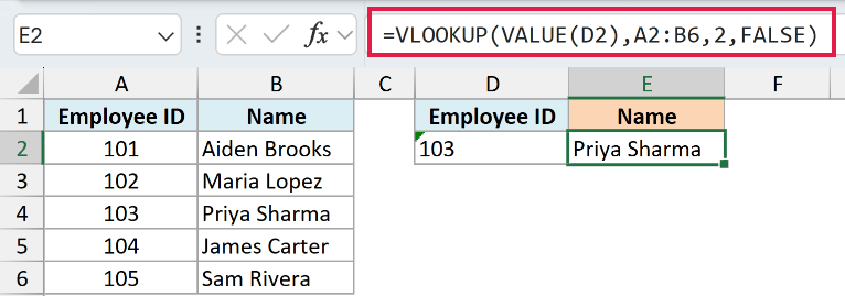
If it’s the reverse, join an empty string to turn the number into text, like VLOOKUP(D2&"", ...). The more permanent fix is to convert the whole column so both sides match, using Text to Columns or Paste Special with Multiply by 1.
5. The Column Index Number Is Wrong or Out of Range
The third argument tells VLOOKUP which column of the table to return, counting from the first column of the table, not from column A of the sheet. Get this number wrong and you either pull the wrong column or trigger an error.
This formula asks for column 3 from a table that only has 2 columns:
=VLOOKUP("Apples",A2:B6,3,FALSE)
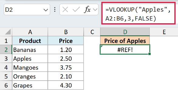
That’s a #REF! error, which is Excel’s way of telling you that you pointed at a column that doesn’t exist.
The fix is to count the columns starting from the table’s first column. In A2:B6, the product is column 1 and the price is column 2, so the right number is 2:
=VLOOKUP("Apples",A2:B6,2,FALSE)
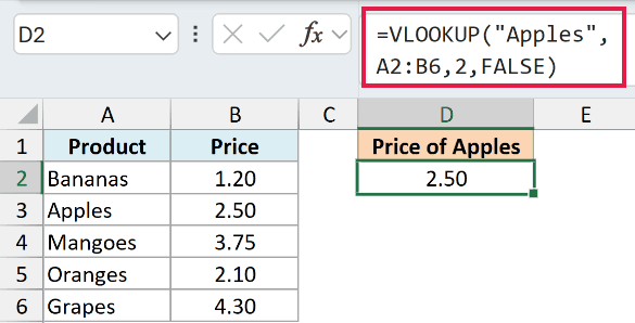
A wrong-but-valid number is trickier, because Excel returns a value with no error at all. So double-check you’re pointing at the column you actually want.
6. The Table Array Isn’t Locked With Dollar Signs
This one bites when you copy a formula down.
If you wrote the table reference as A2:B6 and drag the formula down the column, the range shifts with it, becoming A3:B7, then A4:B8, and your table’s top rows drop out.
=VLOOKUP(D2,A2:B6,2,FALSE)
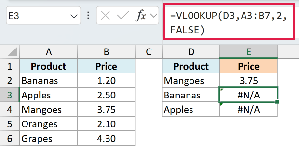
The first row works and the two below it return #N/A. Look at the formula bar: on the second row the range has already slid down to A3:B7, so Bananas is no longer inside the table it’s searching.
The fix is to lock the table with absolute references so it doesn’t move:
=VLOOKUP(D2,$A$2:$B$6,2,FALSE)
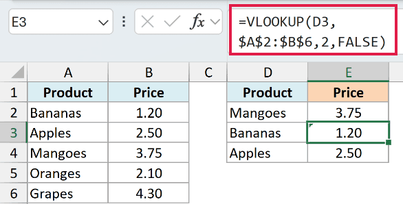
The quick way to add those dollar signs is to click the reference in the formula and press F4. Notice I left D2 without dollar signs, so the lookup value still moves down row by row.
If you want a refresher on when to lock what, here’s my guide on absolute, relative, and mixed references.
7. The Value Genuinely Isn’t There
Sometimes VLOOKUP is working perfectly and the #N/A is telling you the truth: the value really isn’t in the table.
=VLOOKUP(D2,$A$2:$B$6,2,FALSE)
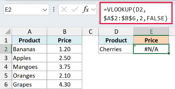
Cherries isn’t in the price list, so #N/A is the correct answer here. Before you do anything else, confirm the value should be there and it isn’t just a typo or a missing row.
If a missing value is a normal, expected thing, you can replace the ugly #N/A with a friendly message using IFERROR:
=IFERROR(VLOOKUP(D2,$A$2:$B$6,2,FALSE),"Not found")
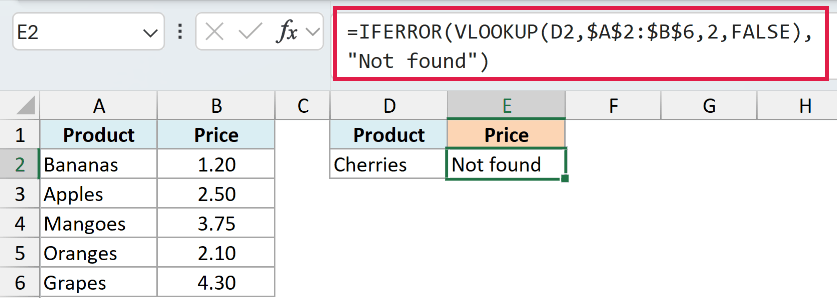
One warning though. IFERROR hides every error, not just the “not there” ones.
If your real problem is stray spaces or a text-versus-number mismatch, IFERROR will quietly show “Not found” and cover up the actual bug. Fix the cause first, then use IFERROR only for values that are legitimately absent.
8. VLOOKUP Ignores Upper and Lower Case
VLOOKUP treats “abc” and “ABC” as the same thing. Usually that’s fine, but if your list has two entries that differ only by case, VLOOKUP returns whichever one comes first, so you get a match, but from the wrong row.
Here I have two product codes that are identical except for their case, and they have different prices.
=VLOOKUP(D2,A2:B4,2,FALSE)
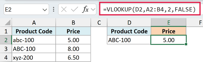
I asked for “ABC-100” and got 5.00, which is the price of the lowercase “abc-100” sitting one row above it. No error, no warning, just the wrong number.
To match the case exactly, use INDEX and MATCH together with EXACT:
=INDEX(B2:B4,MATCH(TRUE,EXACT(D2,A2:A4),0))
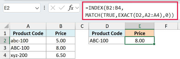
EXACT compares the case exactly and returns TRUE only on the true match, so this correctly returns 8.00.
In Excel 2019 and earlier, enter it with Ctrl + Shift + Enter since it’s an array formula. In 365 and 2021, just press Enter. XLOOKUP is case-insensitive too, so it has the same blind spot.
9. The Lookup Table Is on Another Sheet
When your table lives on a different sheet, you have to tell VLOOKUP where to find it. Leave the sheet reference out, and Excel searches the current sheet instead and comes up empty.
=VLOOKUP(D2,A2:B6,2,FALSE)
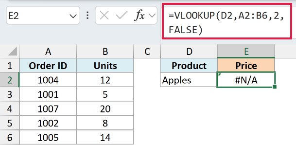
My price list is on a sheet called Price List, but the formula just says A2:B6. So Excel looked at A2:B6 on the sheet I’m sitting on, which holds an order list, found no Apples in it, and returned #N/A.
Mistype the sheet name instead and Excel shows a #REF! error, or pops up a dialog asking you to locate a workbook with that name.
Include the sheet name before the range, followed by an exclamation mark. If the sheet name has spaces in it, wrap the name in single quotes:
=VLOOKUP(D2,'Price List'!$A$2:$B$6,2,FALSE)
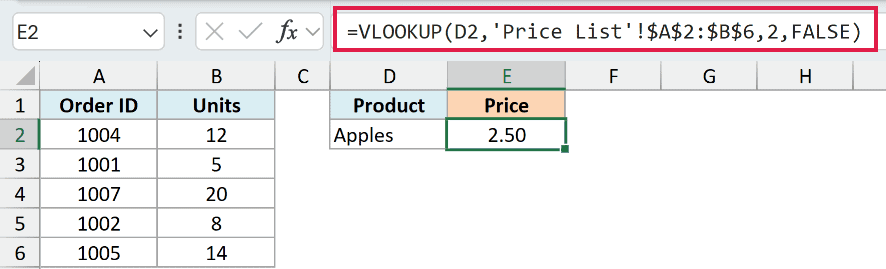
The easiest way to avoid a typo is to start typing the formula, then click the other sheet’s tab and select the range with your mouse. Excel builds the sheet reference for you, quotes and all.
10. Approximate Match on Unsorted Data
Sometimes you actually want an approximate match, like matching a sales figure to a commission tier.
That’s a valid use of VLOOKUP, but it has a strict requirement: the first column has to be sorted in ascending order. If it isn’t, the result is unreliable.
=VLOOKUP(7000,A2:B5,2,TRUE)
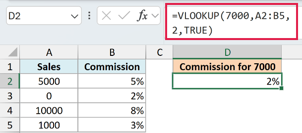
This commission table is scrambled, and the formula returns 2%. That’s the bottom tier, the one for sales starting at 0. The right answer for 7000 is the 5% tier.
Sort the first column smallest to largest (Data, then Sort A to Z) and run exactly the same formula again:
=VLOOKUP(7000,A2:B5,2,TRUE)
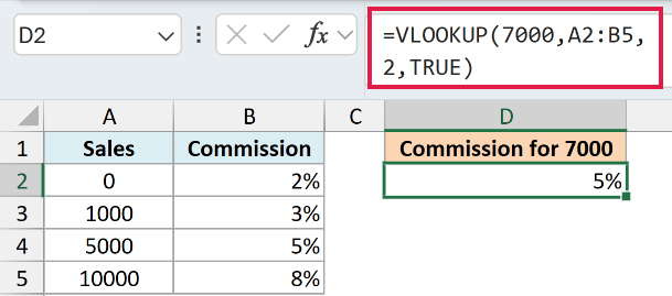
Now it returns 5%, because 5000 is the largest starting value at or below 7000. Same formula, same lookup value, different answer, and the only thing that changed was the sort order.
Or switch to FALSE if you meant to do an exact match all along.
Things to Keep in Mind
- Work from the top of the list down. The exact-match reasons (spaces, text-versus-numbers, wrong column) cause most #N/A errors, so check those before anything fancier.
- Don’t reach for IFERROR too early. It’s great for values that are genuinely missing, but on a broken formula it just hides the real problem instead of fixing it.
- Consider XLOOKUP if you have it. On Excel 365 and 2021, XLOOKUP sidesteps a few of these issues on its own, since it defaults to exact match and can look left.
If you’ve worked through all ten and your formula still won’t cooperate, the issue might be something more general than VLOOKUP itself.
My guide on Excel formulas not working covers the wider culprits, like calculation set to manual or numbers stored as text across the whole sheet.
I hope you found this article helpful.
Other Excel Articles You May Also Like:
