

VLOOKUP (vertical lookup) searches down the first column of a table and returns a value from the same row.
If you want to look up a value in one column and pull back a matching value from another column, the VLOOKUP function is what you reach for. But there is one catch that trips people up on day one.
VLOOKUP only looks to the right. The value you search for has to sit in the leftmost column of your table, and VLOOKUP can only return something from a column to its right.
It also defaults to an approximate match, so a small habit early on saves you a lot of wrong results.
Nothing to worry about though. Once you know these two rules, VLOOKUP is easy to use. In Excel 365 you can even feed it a range of lookup values or an array of column numbers, and the results spill into the neighboring cells.
In this article I’ll show you how to use VLOOKUP with practical examples, from a simple exact match to wildcards, two-way lookups, multiple criteria, case-sensitive matches, and returning several columns at once.
Follow along with the example file
VLOOKUP Function Examples.xlsx
VLOOKUP Syntax
Here is the syntax of the VLOOKUP function:
=VLOOKUP(lookup_value, table_array, col_index_num, [range_lookup])
- lookup_value – The value you want to find. It must be in the first (leftmost) column of your table.
- table_array – The range that holds both the lookup column and the value you want back. The lookup column must be the leftmost one.
- col_index_num – The column number in that range that holds the value to return. The first column is 1, the next is 2, and so on.
- range_lookup – Optional. Use FALSE (or 0) for an exact match, or TRUE (or 1) for an approximate match. If you leave it out, Excel assumes TRUE, which is why so many lookups quietly return the wrong value.
VLOOKUP works in Excel for Microsoft 365, Excel 2024, 2021, 2019, 2016, and Excel on the web.
When to Use VLOOKUP in Excel
Use VLOOKUP when you need to:
- Pull a price, rate, or detail from a reference table using an ID or name.
- Match a value against sorted brackets, like a tiered price or a tax band.
- Replace manual “find the row and copy the value” work with one formula.
Let me show you a few practical examples of how VLOOKUP works.
Example 1: VLOOKUP With an Exact Match
Let’s start with the most common use of VLOOKUP: finding an exact match.
Below is a small cafe menu with the drink name in column A and its price in column B.
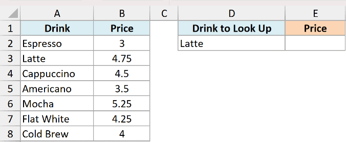
I want to type a drink name in cell D2 and have Excel return its price from the menu.
Here is the formula:
=VLOOKUP(D2,$A$2:$B$8,2,FALSE)
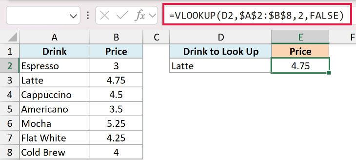
With “Latte” in D2, this returns 4.75.
Here is what each part does. VLOOKUP takes the value in D2, finds it in the first column of the range A2:B8, then returns the value from column 2 of that range (the price).
The FALSE at the end is the important bit. It tells VLOOKUP to find an exact match and return #N/A if the drink isn’t on the menu. Get in the habit of always adding FALSE for this kind of lookup.
Pro Tip: If you have Excel 365 or 2021, use XLOOKUP instead of VLOOKUP. It is cleaner (no column counting), looks up in either direction, and uses an exact match by default. VLOOKUP is still worth knowing for older versions and shared files, which is why this article covers it in full.
Example 2: VLOOKUP With an Approximate Match
Now let’s use the other mode. Approximate match is great for looking a number up against sorted brackets.
Below is a volume pricing table. Column A has the minimum quantity for each tier, and column B has the unit price at that tier. The quantities are sorted from smallest to largest, which matters here.
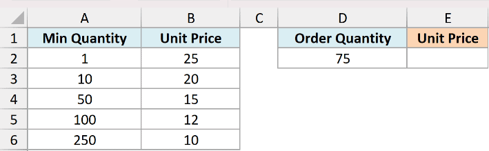
I want to find the unit price for an order of 75 units, which should fall into the 50-unit tier.
Here is the formula:
=VLOOKUP(D2,$A$2:$B$6,2,TRUE)
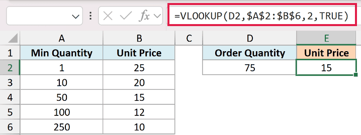
With 75 in D2, this returns 15.
Because the last argument is TRUE, VLOOKUP doesn’t need an exact match. It finds the largest value in column A that is still less than or equal to 75, which is 50, and returns the price on that row.
This is why the table has to be sorted in ascending order. If the quantities were out of order, an approximate match could grab the wrong tier and you would never see an error.
Pro Tip: Approximate match works with a lookup column sorted in ascending numerical or alphabetical order. For names, IDs, or any text where you need an exact match, always use FALSE.
Pro Tip: Use =VLOOKUP(9.99999999999999E+307,$A$2:$A$14,1,TRUE) to get the last number. The lookup value exceeds every number in the column, so approximate match settles on the last. Try the download’s “Last Number” sheet, where it returns 24. Text below it is ignored.
Example 3: Handle #N/A Errors With IFERROR
Here’s a common frustration. When VLOOKUP can’t find the lookup value, it returns #N/A, which looks messy on a report.
I’m using the same cafe menu again, with the drink name in column A and its price in column B.
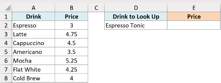
I want to look up a drink in D2, but show a friendly message instead of #N/A when it isn’t on the menu.
Here is the formula:
=IFERROR(VLOOKUP(D2,$A$2:$B$8,2,FALSE),"Not on the menu")
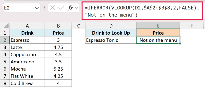
With “Espresso Tonic” in D2 (which isn’t on the menu), this returns “Not on the menu”.
IFERROR runs the VLOOKUP first. If it works, you get the price. If VLOOKUP returns any error, IFERROR shows your text instead.
This keeps dashboards and printouts clean. You can swap the message for anything, or use “” to leave the cell blank when there’s no match.
Example 4: VLOOKUP Across Different Sheets
VLOOKUP doesn’t care which sheet your table lives on. This is handy when your raw data sits on one sheet and your working area is on another.
On a sheet named Products, I have the product ID in column A, the product name in column B, and the price in column C.
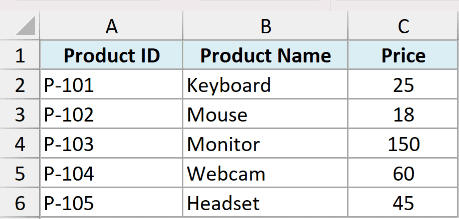
On my Orders sheet, I have a product ID in cell A2, and I want to pull its price from the Products sheet.
Here is the formula:
=VLOOKUP(A2,Products!$A$2:$C$6,3,FALSE)
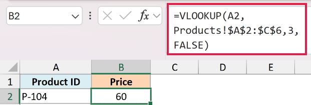
With “P-104” in A2, this returns 60.
The only new part is the Products! in front of the range. That is just the sheet name followed by an exclamation mark, telling VLOOKUP to look in that sheet.
The easiest way to add it is to start typing the formula, then click the other sheet’s tab and select the range with your mouse. Excel writes the sheet reference for you.
Example 5: Partial Match Using Wildcards
Sometimes you only remember part of what you’re looking for. VLOOKUP can match on a piece of text using wildcards.
Below is a short book list with the title in column A and the author in column B.
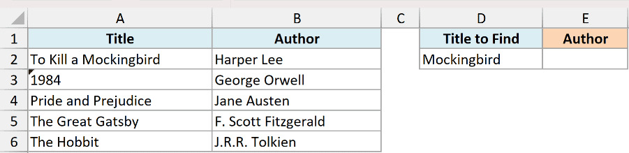
I only remember the word “Mockingbird” from a title, and I want to find its author.
Here is the formula:
=VLOOKUP("*"&D2&"*",$A$2:$B$6,2,FALSE)
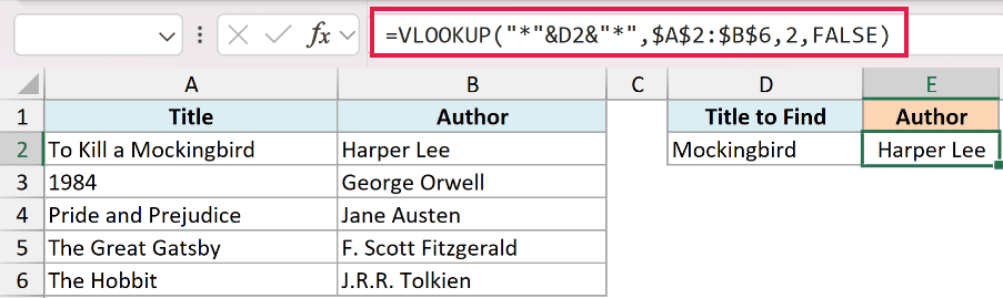
With “Mockingbird” in D2, this returns “Harper Lee”.
The asterisk (*) stands for any number of characters. By wrapping D2 with an asterisk on each side, you’re telling VLOOKUP to match any title that contains “Mockingbird” anywhere inside it.
Wildcards only work when the last argument is FALSE. Use ? to match a single character, and put a tilde (~) before a literal * or ? if you ever need to search for those symbols themselves.
Follow along with the example file
VLOOKUP Function Examples.xlsx
Example 6: Two-Way Lookup With VLOOKUP and MATCH
Here’s a handy one. Instead of hard-coding the column number, you can let a second lookup value pick the column for you.
Below is a small scoreboard with student names in column A and their marks for four subjects across columns B to E.

I want to type a student name in G2 and a subject in H2, and pull back that exact score.
Here is the formula:
=VLOOKUP(G2,$A$2:$E$5,MATCH(H2,$A$1:$E$1,0),0)
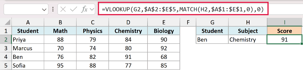
With “Ben” in G2 and “Chemistry” in H2, this returns 91.
The new part is MATCH in place of a fixed column number. MATCH looks up the subject in the header row A1:E1 and returns its position. “Chemistry” sits in the 4th column, so MATCH returns 4.
VLOOKUP then uses that 4 as its col_index_num, so the column updates on its own whenever you change the subject. Change either input and the score follows.
Pro Tip: Pair this with two drop-down lists in G2 and H2 (one for names, one for subjects) and you have a tiny dashboard. A teacher can pick a student and subject from the menus and read the score with no typing.
Example 7: VLOOKUP With Multiple Criteria
Sometimes one lookup value isn’t enough to point at a single row. The trick is to combine your criteria into one key.
Below is a sales table with the rep in column B, the quarter in column C, and sales in column D. Column A is left free for a helper key.
The rep name repeats across quarters, so the name alone can’t pin down one row.
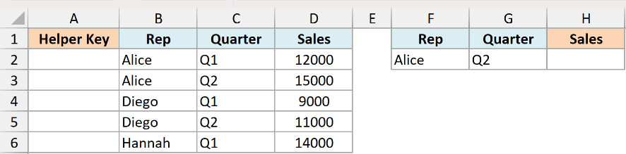
I want Alice’s Q2 sales, matching on both the rep and the quarter at once.
First, build the helper key in column A by joining the two columns with a separator:
=B2&"|"&C2
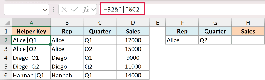
This turns each row into a unique value like “Alice|Q2”. Now VLOOKUP has something single to match against.
Here is the lookup formula, joining the two criteria the same way:
=VLOOKUP(F2&"|"&G2,$A$2:$D$6,4,0)
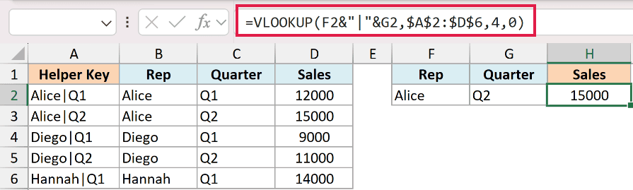
With “Alice” in F2 and “Q2” in G2, this returns 15000.
The formula builds the same “Alice|Q2” key from your two inputs, finds it in column A, and returns the sales from column 4. The separator matters. It prevents ambiguous keys as long as that separator does not occur in either value.
Pro Tip: On Excel 365 you can skip the helper column entirely with XLOOKUP, joining the ranges inside the formula: =XLOOKUP(F2&"|"&G2,$B$2:$B$6&"|"&$C$2:$C$6,$D$2:$D$6). See VLOOKUP with multiple criteria for more on both approaches.
Example 8: Case-Sensitive Lookup With VLOOKUP
By default VLOOKUP ignores case, so “jsmith”, “JSMITH”, and “JSmith” all look the same to it. It returns the first one it hits. Here’s how to make it care about case.
Below is a table of case-sensitive user IDs in column A and the department each one belongs to in column B.
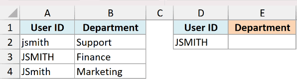
I want the department for the exact ID “JSMITH”, not for “jsmith” or “JSmith”.
Here is the formula:
=VLOOKUP(1,CHOOSE({1,2},--EXACT(D2,$A$2:$A$4),$B$2:$B$4),2,0)
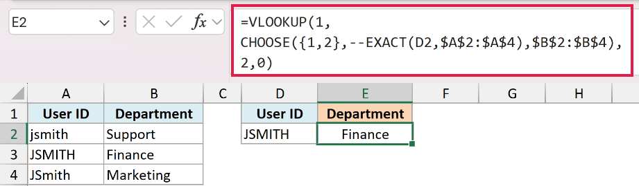
With “JSMITH” in D2, this returns Finance.
How this formula works:
- EXACT(D2,$A$2:$A$4) compares your value to each ID with case, returning {FALSE;TRUE;FALSE}. The
--turns that into {0;1;0}. - CHOOSE({1,2}, … , $B$2:$B$4) stitches those 1s and 0s and the departments into a two-column virtual table for VLOOKUP.
- VLOOKUP(1, … ,2,0) finds the single 1 in the first column and returns the department beside it.
On Excel 365, 2021, or 2024 this works with a plain Enter. On Excel 2019 or earlier, confirm it with Control + Shift + Enter so it evaluates as an array.
Pro Tip: On Excel 365 or 2021, XLOOKUP does this more cleanly with no helper array: =XLOOKUP(TRUE,EXACT(D2,$A$2:$A$4),$B$2:$B$4). It matches the first exact-case ID and returns its department.
Example 9: Return Multiple Columns at Once
Here’s a modern one. In Excel 365, you can pull several columns back with a single VLOOKUP by handing it an array of column numbers.
Below is a product table with the name in column A, category in column B, price in column C, and stock count in column D.
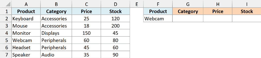
I want to look up one product in F2 and return its category, price, and stock all at once.
Here is the formula:
=VLOOKUP(F2,$A$2:$D$7,{2,3,4},FALSE)
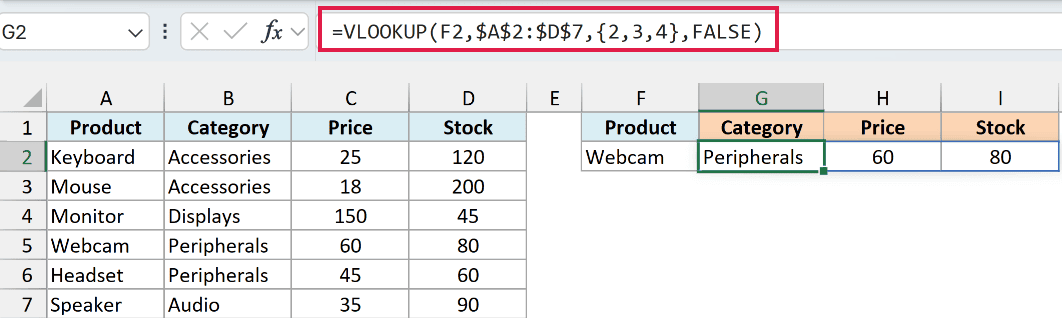
With “Webcam” in F2, this returns Peripherals, 60, and 80, spilling across three cells.
Instead of one column number, you give VLOOKUP an array in curly braces, {2,3,4}. It returns column 2, 3, and 4 for the match, and the results spill into the cells to the right.
This spill works in Microsoft 365, Excel 2021, and Excel 2024. In older versions you would write a separate VLOOKUP for each column, changing the col_index_num each time.
Example 10: Getting Around the Left-Lookup Limit
This is the wall most people hit. VLOOKUP can only return values to the right of the lookup column, so what if the value you want is on the left?
Below is an orders table with the Order ID in column A and the Customer in column B.
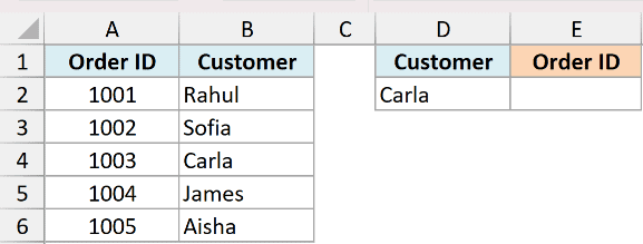
I know the customer name in D2 and I want their Order ID, which sits in the column to the left. A plain VLOOKUP can’t do this.
The clean fix is XLOOKUP, which looks in either direction:
=XLOOKUP(D2,$B$2:$B$6,$A$2:$A$6)
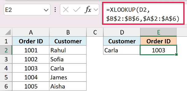
With “Carla” in D2, this returns 1003.
XLOOKUP takes the value to find, the range to search, and the range to return from. Because you point at each range yourself, it happily looks left.
If you’re on an older version without XLOOKUP, the classic workaround is INDEX and MATCH, which can also return a value from any column, left or right.
Tips & Common Mistakes
- Always add FALSE for exact lookups. If you leave the last argument out, VLOOKUP defaults to an approximate match and can return a wrong-but-plausible value with no error.
- The lookup value must be in the leftmost column. VLOOKUP only looks to the right. To return a value from a column on the left, use XLOOKUP or INDEX and MATCH.
- Lock the table_array with $ signs. Use an absolute reference like
$A$2:$B$8so the range doesn’t shift when you copy the formula down. - #N/A means no match was found. Check for extra spaces, a number stored as text, or a lookup value that genuinely isn’t there. Wrap it in IFERROR to show a cleaner message.
- col_index_num counts within the table, not the sheet. Column 1 is the first column of your range, not column A of the worksheet.
- Matching on more than one column? Combine your criteria into a single helper key as in Example 7, or use the helper-free approach in VLOOKUP with multiple criteria.
- No IFERROR on a very old version? IFERROR arrived in Excel 2007. On Excel 2003 or earlier, catch #N/A with
=IF(ISERROR(VLOOKUP(...)),"Not found",VLOOKUP(...))instead. - Prefer XLOOKUP for new work. If you’re on Excel 365 or 2021, XLOOKUP is the cleaner, bidirectional replacement. Keep VLOOKUP for older versions and files shared with people who don’t have it.
That covers the ways I actually use VLOOKUP day to day, from a plain exact match to wildcards, two-way and multi-criteria lookups, and returning several columns at once. Get comfortable with the FALSE-for-exact-match habit and the leftmost-column rule, and the rest falls into place quickly.
If you’re on a recent version of Excel, learn XLOOKUP next. It does everything here with less fuss, and you’ll rarely reach for VLOOKUP again.
Other Excel Articles You May Also Like:
