

If you want to find where a specific character or word sits inside a text string, the FIND function gives you its exact position as a number.
It is case-sensitive, so it treats uppercase and lowercase letters as different characters. In Excel 365, you can also feed FIND a range and the results spill into the cells below.
In this article, I’ll show you how to use FIND to locate characters, pull out parts of a text string, and handle the cases where the text you’re looking for isn’t there.
FIND Syntax
Here is the syntax of the FIND function:
=FIND(find_text, within_text, [start_num])
- find_text – The text or character you want to locate.
- within_text – The text string you want to search inside.
- [start_num] – Optional. The character position where the search starts. If you leave it out, FIND starts at the first character.
When to Use the FIND Function
Use FIND when you need to:
- Get the position of a character or word inside a longer text string
- Pull out part of a text string by combining it with LEFT, MID, or RIGHT
- Locate a delimiter (like @, a dash, or a space) so you can split text around it
- Run a case-sensitive search where uppercase and lowercase must be treated differently
Let me show you a few practical examples of how to use this function.
Example 1: Find the Position of a Character in a Text String
Let’s start with a simple example.
Below is a dataset with a list of file names in column A. Each name has a dot before the file extension.
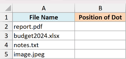
I want to know the position of the dot in each file name.
Here is the formula:
=FIND(".",A2:A5)
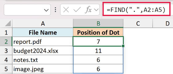
FIND returns the position of the first period in each file name. Because I fed it the whole range A2:A5 in Excel 365, the single formula spills a result down the column, one number per file name.
So report.pdf returns 7 and budget2024.xlsx returns 11, since the dot sits further along in that longer name.
Pro Tip: FIND always stops at the first match. If a character appears more than once, you get the position of the first one, not the last. I’ll show you how to reach later matches in Examples 5 and 7.
Example 2: FIND Is Case-Sensitive (FIND vs SEARCH)
Here’s something important to know about FIND.
Below is a dataset with three text labels in column A, each with a capital and a lowercase “s”.
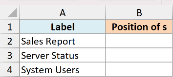
I want to find the position of the lowercase “s” in each label.
Here is the formula:
=FIND("s",A2:A4)
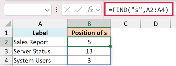
Notice that FIND skips the capital “S” at the start of “Sales Report” and returns 5, the position of the first lowercase “s”. That’s because FIND is case-sensitive and treats “S” and “s” as different characters.
Now compare that with SEARCH, which is not case-sensitive. Here is the formula:
=SEARCH("s",A2:A4)
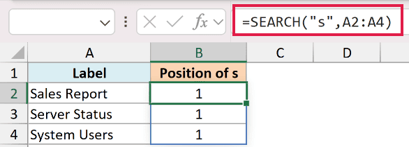
SEARCH ignores case, so it matches the capital “S” first and returns 1 for “Sales Report” and “Server Status”. This is the key difference between the two functions.
Pro Tip: If you want a search that ignores case, use the SEARCH function instead of FIND. SEARCH also lets you use wildcards, which FIND does not.
Example 3: Extract the Username Before a Delimiter (FIND + LEFT)
Now let’s use FIND to pull out part of a text string.
Below is a dataset with a list of email addresses in column A.
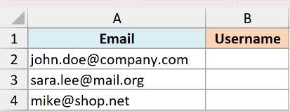
I want to extract just the username, which is everything before the @ sign.
Here is the formula:
=LEFT(A2:A4,FIND("@",A2:A4)-1)
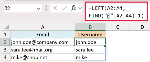
How this formula works:
- FIND locates the position of the @ sign in each email address.
- Subtracting 1 gives the position of the last character before the @.
- The LEFT function then pulls that many characters from the start of the text.
So john.doe@company.com returns john.doe.
Example 4: Extract the Domain After a Delimiter (FIND + MID)
Here’s the reverse of the last example.
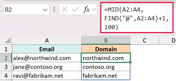
Below is a dataset with email addresses that use different domains in column A.
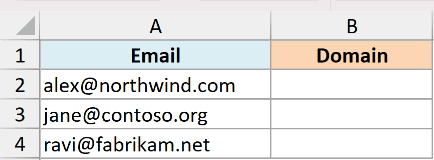
This time I want the domain, which is everything after the @ sign.
Here is the formula:
=MID(A2:A4,FIND("@",A2:A4)+1,100)
How this formula works:
- FIND gives the position of the @ sign, and adding 1 moves one character past it.
- The MID function starts pulling text from that position.
- The 100 is just a number large enough to grab the rest of the string, however long the domain is.
So alex@northwind.com returns northwind.com.
Example 5: Find the Nth Occurrence of a Character
This next one is handy when a character shows up more than once.
Below is a dataset with reference codes in column A. Each code has two dashes.
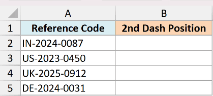
I want to find the position of the second dash, not the first.
Here is the formula:
=FIND("-",A2,FIND("-",A2)+1)
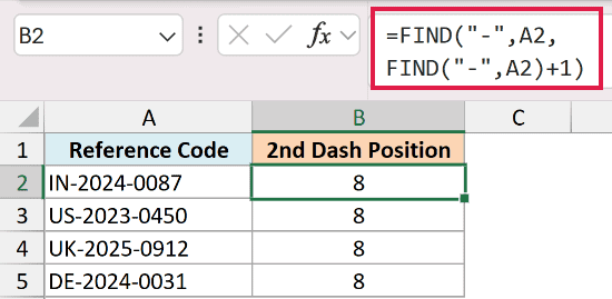
The inner FIND locates the first dash. Adding 1 to that position, and passing it as the start_num argument to the outer FIND, tells FIND to start searching just after the first dash.
So for IN-2024-0087, the first dash is at position 3 and the second dash is at position 8.
We keep this one as a per-row formula because the nested FIND reads most clearly against a single cell. In Excel 365 you can also feed it the whole range to spill the results.
Example 6: Handle Not-Found Errors with IFERROR
FIND returns an error when the character isn’t there, so let’s deal with that.
Below is a dataset in column A that mixes email addresses and phone numbers.
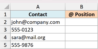
I want the position of the @ sign, but only the email rows have one.
Here is the formula:
=FIND("@",A2:A5)
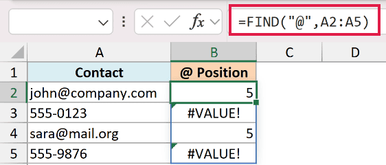
The email rows return 5, but the phone-number rows return a #VALUE! error because FIND can’t find an @ in them.
To replace that error with a friendly message, wrap the formula in IFERROR. Here is the formula:
=IFERROR(FIND("@",A2:A5),"No email")
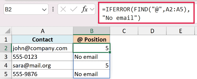
Now the phone-number rows show “No email” instead of an error, while the email rows still return the @ position. IFERROR catches the #VALUE! and returns whatever you put in its second argument.
Example 7: Find the Last Occurrence of a Character
Let’s finish with a common one: finding the last time a character appears.
Below is a dataset with folder paths in column A. Each path uses forward slashes, and I want the position of the last slash.
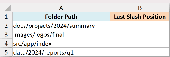
FIND on its own only reaches the first slash, so I’ll combine it with SUBSTITUTE to jump to the last one.
Here is the formula:
=FIND("~",SUBSTITUTE(A2,"/","~",LEN(A2)-LEN(SUBSTITUTE(A2,"/",""))))
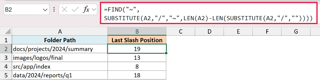
How this formula works:
LEN(A2)-LEN(SUBSTITUTE(A2,"/",""))counts how many slashes are in the text.- The SUBSTITUTE function then swaps only that last slash for a marker character (~).
- FIND locates the marker, which is exactly the position of the last slash.
So for docs/projects/2024/summary, the formula returns 19, the position of the third and final slash.
Pro Tip: Pick a marker character (like ~) that doesn’t already appear anywhere in your text. If the marker exists in the string, FIND could land on the wrong one.
Tips & Common Mistakes
- FIND is case-sensitive. Searching for “a” won’t match “A”. When case shouldn’t matter, use the SEARCH function instead.
- FIND returns #VALUE! when the text isn’t found. Wrap it in IFERROR to show a message of your choice instead of an error.
- FIND does not support wildcards. If you need to match patterns with * or ?, use SEARCH, which does support wildcard characters.
- FIND only returns the first match. To reach a later one, use the start_num argument (Example 5) or the SUBSTITUTE marker trick (Example 7).
- Positions count from 1. The first character in the text is position 1, not 0.
FIND is one of those small functions that quietly powers a lot of text work in Excel. On its own it just returns a position, but paired with LEFT, MID, RIGHT, IFERROR, or SUBSTITUTE it becomes the tool you reach for whenever you need to split, extract, or clean up text.
Try it on your own data and you’ll find plenty of places it saves you a manual edit.
Other Excel Articles You May Also Like: