

If you want the arithmetic mean of a set of numbers in Excel, the AVERAGE function is the fastest way to get it. You hand it a range and it returns the mean in a single cell.
There is one thing worth knowing up front. AVERAGE ignores blank cells and text, but it still counts any cell that holds a zero, and that can quietly pull your result down.
AVERAGE returns a single value, but it works seamlessly inside dynamic array formulas like =AVERAGE(FILTER(...)). In this article I’ll show you how to use AVERAGE in Excel, from a basic mean to averaging non-contiguous cells, skipping errors, and getting a conditional average.
AVERAGE Syntax
Here is the syntax of the AVERAGE function:
=AVERAGE(number1, [number2], ...)
- number1 – The first number, cell reference, or range you want to average. This one is required.
- [number2], … – Optional. Any additional numbers, references, or ranges. You can pass up to 255 arguments in total.
A quick note on how it treats a range: AVERAGE ignores blank cells, text, and logical values (TRUE/FALSE) inside a referenced range. Cells that hold a zero are counted. If the range contains an error value, AVERAGE returns that error.
When to Use AVERAGE
Use the AVERAGE function when you need to:
- Find the mean of a column or row of numbers in one cell.
- Average values sitting in cells that are not next to each other.
- Feed a mean into a bigger formula, like averaging only the rows a FILTER returns.
Let me show you a few practical examples of how AVERAGE works.
Example 1: Get a Basic Average
Let’s start with a simple example.
Below is a dataset with the length of a person’s daily workout, in minutes, for one week. Column A has the day and column B has the minutes.
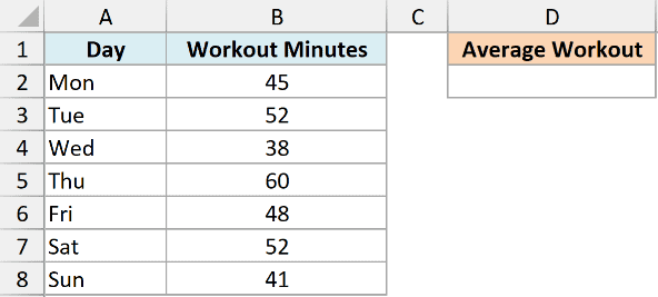
I want the average workout length across the whole week.
Here is the formula:
=AVERAGE(B2:B8)
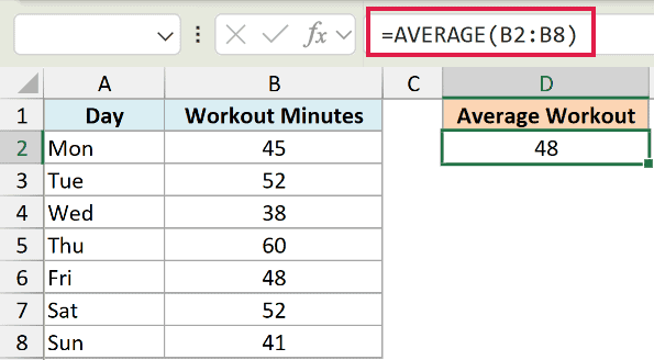
This returns 48, which is the average of the seven daily values. AVERAGE adds up everything in B2:B8 and divides by how many numbers it found, so you don’t have to count the cells yourself.
Example 2: How AVERAGE Handles Blanks vs Zeros
This next one is the mistake I see trip people up the most.
Below is a dataset with the units a salesperson sold each day from Monday to Friday. On Wednesday and Friday the cells are blank, because those were days off with no data recorded.
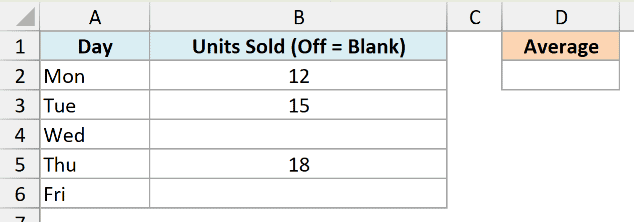
I want the average units sold across the days the person actually worked.
Here is the formula:
=AVERAGE(B2:B6)
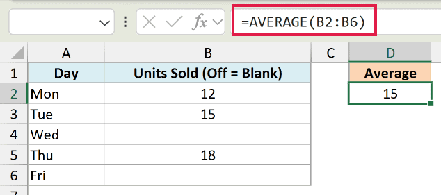
This returns 15. AVERAGE skips the two blank cells entirely, so it adds 12 + 15 + 18 and divides by 3, not by 5.
Now look at what happens when those two days hold a 0 instead of being blank. Same numbers on the working days, but Wednesday and Friday now show a real zero.
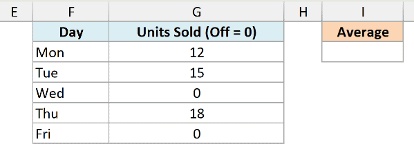
Here is the same formula on that version:
=AVERAGE(B2:B6)
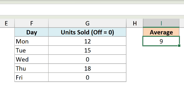
This time it returns 9. AVERAGE counts the two zeros as real values, so it divides the same total of 45 by 5 days instead of 3. A blank and a zero are not the same thing to AVERAGE.
Pro Tip: If you want to ignore zeros as well as blanks, use AVERAGEIF with a “not equal to zero” condition: =AVERAGEIF(B2:B6,”<>0″). It leaves the zeros out and averages only the non-zero numbers.
Example 3: Average Non-Contiguous Cells
Here’s a handy one when the cells you care about are scattered.
Below is a dataset with new sign-ups for each month of the year. Column A has the month and column B has the count.
You launched a new feature only in January, April, July, and October, and those are the rows you want to look at.
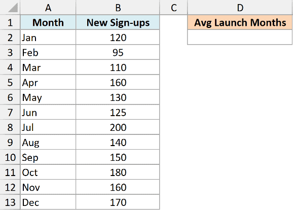
I want the average sign-ups for just those four launch months, ignoring every other row.
Here is the formula:
=AVERAGE(B2,B5,B8,B11)
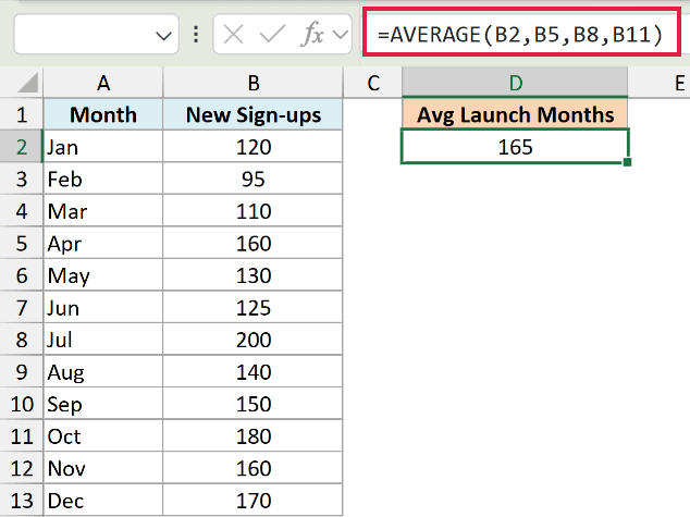
This returns 165. Instead of a single range, you pass each cell as its own argument separated by commas, and AVERAGE means just those four. The values are 120, 160, 200, and 180, which add to 660 and divide by 4.
Example 4: Average and Ignore Error Values
Let’s look at something that catches a lot of dashboards off guard.
Below is a dataset of stores showing their Sales, Visits, and the Sales per Visit ratio in column D (Sales divided by Visits). A couple of stores had no visits that day, so their ratio came out as a #DIV/0! error.
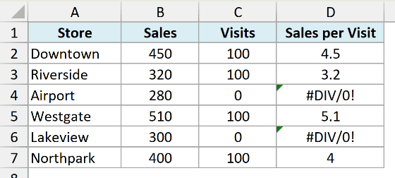
I want the average ratio across the stores that do have a valid number.
Here is the plain AVERAGE formula first:
=AVERAGE(D2:D7)
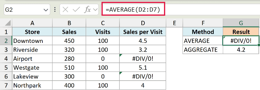
This returns #DIV/0!. A single error anywhere in the range makes AVERAGE hand that same error straight back, which is rarely what you want.
To skip the errors, use the AGGREGATE function instead:
=AGGREGATE(1,6,D2:D7)
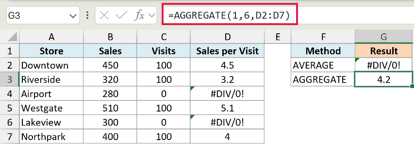
This returns 4.2. In AGGREGATE, the first argument 1 tells it to average, and the second argument 6 tells it to ignore error values. So it averages only the four clean numbers and quietly drops the two errors.
Example 5: Average the Top (or Bottom) N Values
Now let’s combine AVERAGE with another function.
Below is a dataset with the monthly sales for eight reps. Column A has the rep name and column B has their sales number. You don’t want the average of everyone, just your strongest performers.
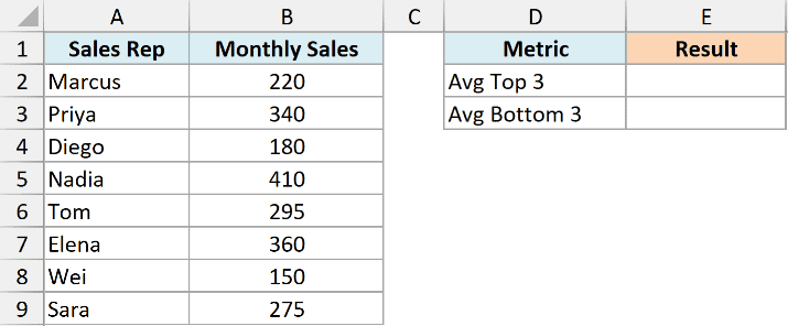
I want the average sales of the top three reps.
Here is the formula:
=AVERAGE(LARGE(B2:B9,{1,2,3}))
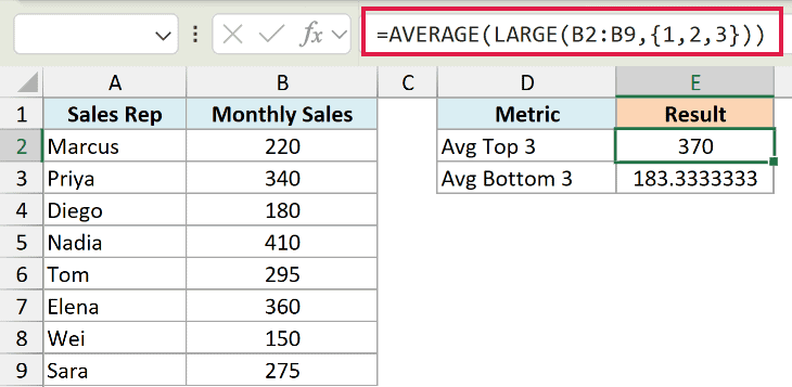
This returns 370. The LARGE function pulls the 1st, 2nd, and 3rd highest values (410, 360, and 340) as a small array, and AVERAGE takes the mean of just those three.
You can flip it to the bottom three by swapping in the SMALL function, which grabs the lowest values instead:
=AVERAGE(SMALL(B2:B9,{1,2,3}))
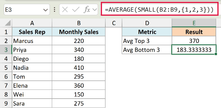
This returns about 183.3, the mean of the three lowest sales (150, 180, and 220). Change the {1,2,3} to {1,2,3,4,5} and you would average the top or bottom five instead.
Example 6: Conditional Average With FILTER
Let’s finish with a modern one that shows how AVERAGE composes with dynamic arrays.
Below is a dataset with orders. Column A has the order ID, column B has the region, and column C has the order amount. Rows for different regions are mixed together in no particular order.
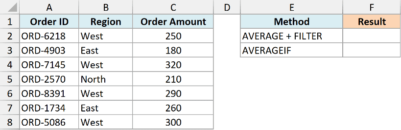
I want the average order amount for the West region only.
Here is the formula:
=AVERAGE(FILTER(C2:C8,B2:B8="West"))
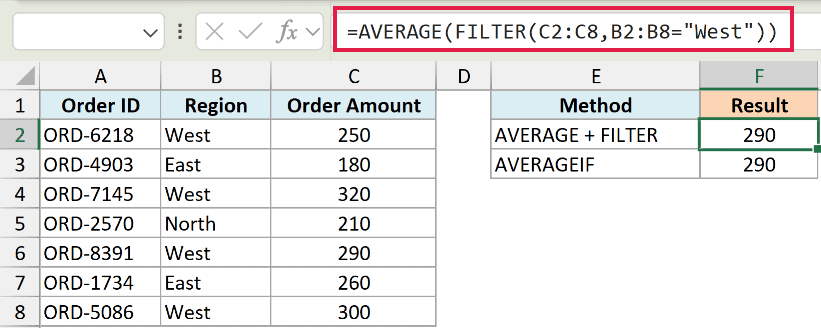
This returns 290. The FILTER function returns just the West amounts (250, 320, 290, and 300) as an array, and AVERAGE reduces that array to a single mean.
This is the composition to remember. AVERAGE never spills on its own, but it happily sits on top of a spilling function.
For a straightforward single-condition average like this, the AVERAGEIF function is usually the cleaner tool and works in every version of Excel:
=AVERAGEIF(B2:B8,"West",C2:C8)
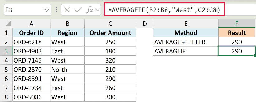
This also returns 290. Reach for AVERAGEIF when you have one condition, the AVERAGEIFS function when you have several, and the FILTER approach when you want to layer more logic into the array first.
Tips & Common Mistakes
- Blanks are ignored, zeros are not. This is the big one. A blank cell is left out of the count, but a cell holding 0 is treated as a real value and drags the mean down. To skip zeros too, use
=AVERAGEIF(range,"<>0"). - Text and logical values in a range are skipped. If a referenced range mixes numbers with text or TRUE/FALSE, AVERAGE just averages the numbers. Note that TRUE/FALSE typed directly as arguments (not in a range) are counted as 1 and 0.
- One error breaks the whole result. If any cell in the range is an error like
#N/Aor#DIV/0!, AVERAGE returns that error. Use=AGGREGATE(1,6,range)to average and ignore the errors. - AVERAGE is a reducer, not a spilling function. It collapses a range to one number, so it won’t spill on its own. It does drop cleanly into dynamic array formulas like
=AVERAGE(FILTER(...)). - AVERAGE weights every value equally. If some values should count more than others, a plain average won’t do it. That’s a job for a weighted average built with SUMPRODUCT.
That covers the AVERAGE function from a basic mean to the zero-versus-blank gotcha, non-contiguous cells, skipping errors, averaging the top values, and a conditional average with FILTER. Once you know that AVERAGE ignores blanks but counts zeros, most of the surprises go away.
Pick the example closest to your data and adapt the range, and you’ll have your mean in seconds.
Other Excel Articles You May Also Like:
