

With the ROUNDUP function in Excel, you can round a number up to the decimal places you choose, a whole number, or the nearest thousand. It always rounds away from zero, so the result is never smaller in size than the number you started with.
That makes it the right choice when coming up short isn’t an option, like splitting a bill or charging for time in full hours.
In this article, I’ll show you how to use ROUNDUP with seven examples, including working out how many packs to buy, handling negative numbers, and rounding time up to the next hour.
Follow along with the example file
ROUNDUP Function Examples.xlsx
ROUNDUP Function Syntax
Here is the syntax of the ROUNDUP function:
=ROUNDUP(number,num_digits)
- number – The number you want to round up. It can be a typed number, a cell reference, a calculation such as B2/C2, or a whole range.
- num_digits – How many digits to round to.
Both arguments are required, so you always have to tell ROUNDUP how many digits to keep.
A positive num_digits rounds to that many decimal places, so =ROUNDUP(3.14159,2) returns 3.15. A 0 rounds up to the next whole number, so =ROUNDUP(3.14159,0) returns 4.
A negative num_digits rounds to the left of the decimal point. -1 rounds up to the next ten, -2 to the next hundred, and -3 to the next thousand, so =ROUNDUP(1234.5,-2) returns 1300.
The ROUNDUP function works in all Excel versions, including 365, 2024, 2021, 2019, 2016, Mac, and the web.
When to Use the ROUNDUP Function
Use it when you need to:
- Buy whole items or full packs, where a fraction would leave you short.
- Split a bill so the shares add up to at least the total.
- Set a budget or estimate that lands on a clean figure, like the next thousand.
- Bill time in full units, where any part of an hour counts as an hour.
- Turn a month number into a quarter number.
Let me show you a few practical examples of how this works.
Example 1: Round Up to the Nearest Whole Number
Let’s start with a simple example.
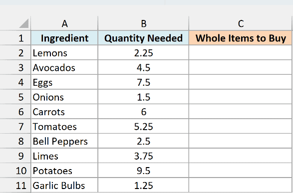
Below is a shopping list with how much of each ingredient a recipe needs, and I want the number of whole items to buy in column C.
Here is the formula:
=ROUNDUP(B2:B11,0)
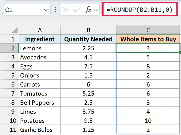
In the above formula, a num_digits of 0 tells ROUNDUP to go to the next whole number. So 2.25 lemons becomes 3, and 4.5 avocados becomes 5.
Notice that Carrots stays at 6. ROUNDUP only changes a number when there’s something to round, so a value that’s already whole comes back as it is.
You enter this formula once in cell C2, and in Excel 365 and 2021 or later it spills the results down to C11. If any of those cells already has something in it, you’ll get a #SPILL! error until you clear it.
If you are using Excel 2019 or earlier, enter the below formula in cell C2 and then copy it down the range:
=ROUNDUP(B2,0)
The same works for every example in this article. Replace each range with its first cell (so B2:B11 becomes B2), enter the formula in the first result cell, and copy it down.
Example 2: Round Up to Two Decimal Places
Here’s another everyday situation, splitting a bill between friends.
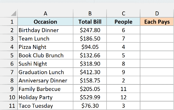
Below are some group bills with the total and the number of people, and I want what each person pays, rounded up to the cent, in column D.
Here is the formula:
=ROUNDUP(B2:B11/C2:C11,2)
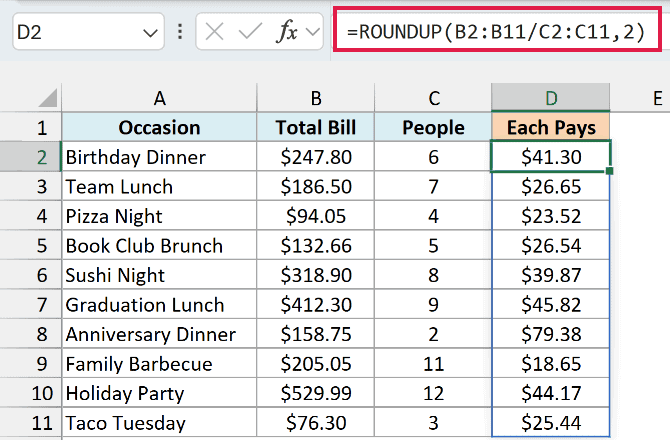
Here, the formula first divides each bill by the number of people, and then ROUNDUP rounds the answer up to two decimal places. For Pizza Night, $94.05 split four ways is $23.5125, and ROUNDUP turns that into $23.52.
Rounding up matters here because everyone’s share has to cover the bill. Four people paying $23.52 gives $94.08, so the bill is covered with a few cents to spare.
Important: Formatting a cell to show two decimals doesn’t round the value up. The currency format would show $23.5125 as $23.51, and four people paying $23.51 leaves the bill one cent short.
Example 3: Round Up to the Nearest Thousand
Now let’s use a negative num_digits to round to the left of the decimal point.
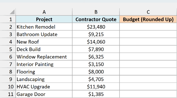
Below are contractor quotes for some home projects, and I want a budget for each one, rounded up to the next thousand, in column C.
Here is the formula:
=ROUNDUP(B2:B11,-3)
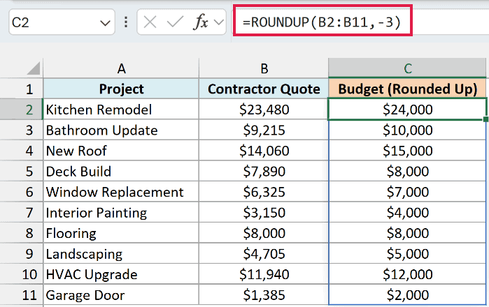
A num_digits of -3 rounds to the thousands place. The Kitchen Remodel quote of $23,480 becomes a $24,000 budget, even though it’s closer to $23,000.
That’s the difference from the ROUND function, which would give you $23,000 and leave the budget below the quote.
Example 4: ROUNDUP With Negative Numbers
This one is about what “up” means when a number is negative, and it’s where ROUNDUP surprises people.
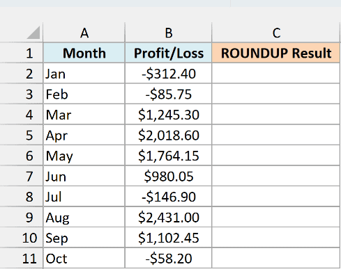
Below is a monthly profit and loss list with a few loss months, and I want each value rounded to a whole dollar with ROUNDUP in column C, and then with CEILING.MATH in column D to compare.
Here is the ROUNDUP formula:
=ROUNDUP(B2:B11,0)
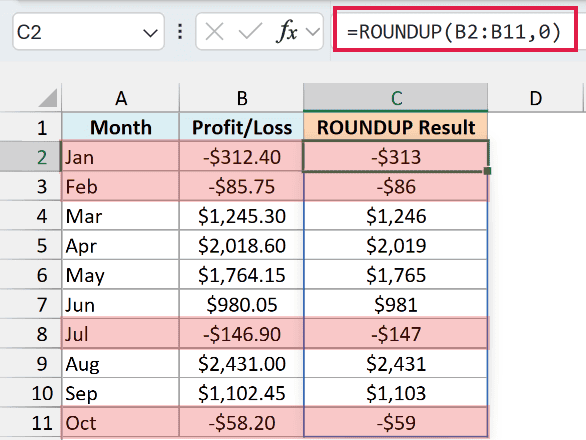
Look at the loss months first. ROUNDUP turns -$312.40 into -$313 and -$85.75 into -$86, because it always rounds away from zero, so a negative number gets more negative.
The positive months behave the way you’d expect, so $1,245.30 becomes $1,246.
Excel has another round-up function, CEILING.MATH, and it treats negative numbers differently. Here is the formula for comparison:
=CEILING.MATH(B2:B11)
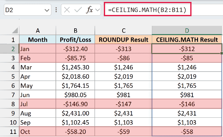
CEILING.MATH rounds toward the larger number instead. That turns -$312.40 into -$312, while every positive month gets the same result as ROUNDUP.
Pick the one that matches what you’re reporting. If you want a loss to show at its full size, ROUNDUP gives you -$313, and if you want the value to move toward the larger number, CEILING.MATH gives you -$312.
If you’d rather have CEILING.MATH round negative numbers away from zero too, set its second argument (significance) to 1 and its third argument (mode) to 1. Then it matches ROUNDUP on this list.
For rounding up to a multiple like the nearest 5 or 0.5, CEILING.MATH is the one to use, because ROUNDUP can’t do that.
Example 5: Calculate How Many Packs to Buy
Now let’s work out how many full packs you need to buy.
Below is a party supply list with how many of each item I need and how many come in a pack, and I want the number of packs to buy in column D.
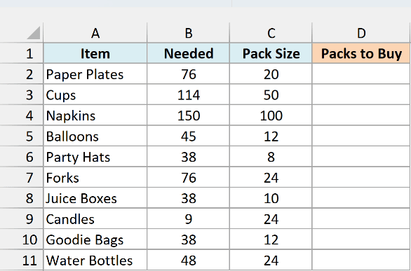
Here is the formula:
=ROUNDUP(B2:B11/C2:C11,0)
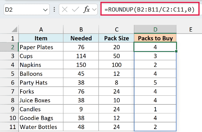
The formula divides what I need by the pack size, then rounds up to a whole pack. Paper Plates need 76 with 20 in a pack, which is 3.8 packs, so I buy 4.
When the numbers divide exactly, no extra pack gets added. 48 water bottles in packs of 24 is exactly 2 packs, and ROUNDUP returns 2.
That’s why ROUNDUP is better here than the shortcut of taking the whole number with the INT function and adding 1. That shortcut works for 3.8, but it would tell you to buy 3 packs of water bottles when 2 is enough.
Example 6: Round Up Time to the Next Full Hour
This next one bills time in full hours, the way a parking garage does.
Below is a parking log with the entry and exit time for each ticket, and I want the billable hours in column D, where any part of an hour counts as a full hour.
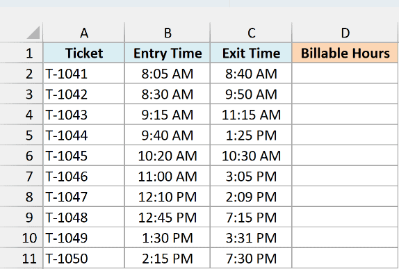
Here is the formula:
=ROUNDUP((C2:C11-B2:B11)*24,0)
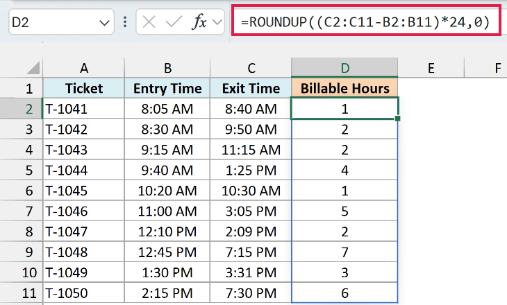
How this formula works:
- C2:C11-B2:B11 subtracts the entry time from the exit time. Excel stores time as a fraction of a day, so 2 hours comes out as 0.0833.
- Multiplying by 24 turns that fraction of a day into hours.
- ROUNDUP(…,0) rounds the hours up to the next whole hour.
Ticket T-1047 was parked for 1 hour 59 minutes, so it’s billed 2 hours. T-1049 stayed 2 hours and 1 minute, and that one extra minute makes it 3 hours.
Example 7: Find the Quarter From a Date
Let’s finish with a neat trick that combines ROUNDUP with the MONTH function.
Below is a list of invoices with their dates, and I want the quarter for each one, like Q1 or Q2, in column C.
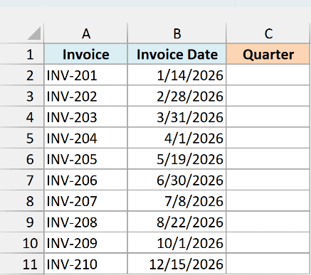
Here is the formula:
="Q"&ROUNDUP(MONTH(B2:B11)/3,0)
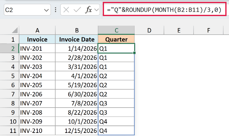
How this formula works:
- MONTH(B2:B11) gets the month number of each date, from 1 for January to 12 for December.
- /3 divides it by 3, since each quarter has three months.
- ROUNDUP(…,0) rounds that up to a whole number, which gives 1, 2, 3, or 4.
- “Q”& joins the letter Q in front of the number.
So April 1 is month 4, and 4 divided by 3 is 1.33, which rounds up to 2 and gives Q2. March 31 is month 3, which is exactly 1, so it stays in Q1.
This works for calendar quarters that start in January. If your fiscal year starts in a different month, you’ll need to shift the month number by that offset before dividing by 3.
So these are seven ways you can use the ROUNDUP function in Excel. Use it whenever coming up short isn’t an option, and remember that with negative numbers, “up” means further from zero.
I hope you found this article helpful.
Other Excel Articles You May Also Like:
