

The MONTH function in Excel returns the month of a date as a number from 1 (January) to 12 (December). It’s useful when you want to group or total data by month, or work out the quarter or fiscal year a date falls in.
In this article, I’ll show you how to use MONTH with eight examples, including getting the month name, fixing blank cells that return 1, and summing values by month.
Follow along with the example file
MONTH Function Examples.xlsx
MONTH Function Syntax
Here is the syntax of the MONTH function:
=MONTH(serial_number)
- serial_number – The date you want the month from. This is usually a cell with a date in it, but it can also be a date returned by another formula, or a whole range of dates.
MONTH only looks at the date part. A cell that holds 3/14/2026 5:30 PM still returns 3, so you don’t need to strip out the time first.
You can also type a date straight into the formula in quotes, so =MONTH("15-Mar-2026") returns 3. But an all-number date like “03/04/2026” is read using your computer’s regional settings, so it means March 4 in the US and April 3 in the UK.
That’s why it’s safer to point MONTH at a cell that holds a real date. If the date doesn’t live in a cell, build it with the DATE function instead, as in =MONTH(DATE(2026,3,4)).
The MONTH function works in all Excel versions, including 365, 2024, 2021, 2019, 2016, Mac, and the web.
When to Use the MONTH Function
Use this function when you need to:
- Pull the month number out of a date so you can sort, filter, or group by month
- Work out which quarter or fiscal year a date falls in
- Add up or count values for one particular month
- Get the first day of the month for any date
- Turn a month name like “June” into its number
Let me show you a few practical examples of how to use the MONTH function.
Example 1: Get the Month From a Date in Excel
Let’s start with the simplest use.
Below is a library loan log with the date each book was borrowed, and I want to get the month number in column C.
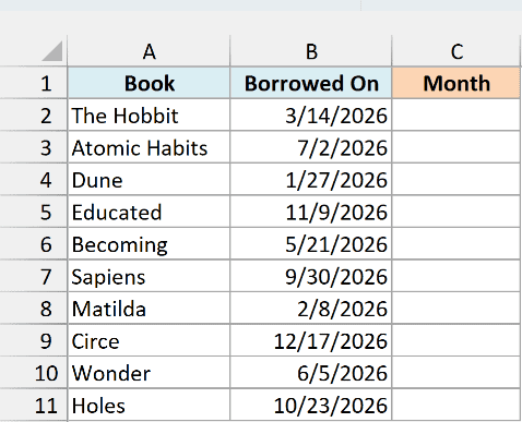
Here is the formula:
=MONTH(B2:B11)
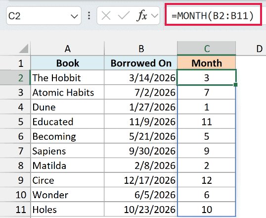
In the above formula, I’ve given MONTH the whole range of dates (B2:B11) instead of one cell. It returns one month number for each date, and the results spill into C2:C11 by themselves.
So The Hobbit, borrowed on 3/14/2026, gets 3, and Circe, borrowed on 12/17/2026, gets 12.
The spill needs the cells below C2 to be empty. If anything is sitting in C3:C11, you get a #SPILL! error instead of the results, and clearing those cells fixes it.
If you are using Excel 2019 or earlier, enter the below formula in cell C2 and then copy it down to C11:
=MONTH(B2)
The same goes for Examples 2 to 7, which also fill a column. In older versions, point each formula at the first cell (B2 instead of B2:B11) and copy it down.
Example 2: Get the Month Name From a Date
A month number works well inside formulas, but in a report you usually want the name.
MONTH can’t do this on its own, because it only ever returns a number. To get the name, you use the TEXT function on the date itself.
Below is the same loan log, and this time I want the full month name, like March, in column C.
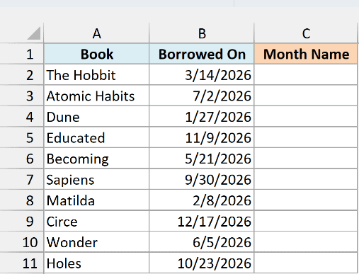
Here is the formula:
=TEXT(B2:B11,"mmmm")
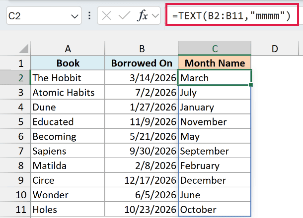
The format code “mmmm” tells the TEXT function to show the full month name of each date. If you want the short version (Mar, Jul), use “mmm” instead.
Now here’s the version you might try first, wrapping MONTH inside TEXT. I’ve put it in column D so you can compare the two:
=TEXT(MONTH(B2:B11),"mmmm")
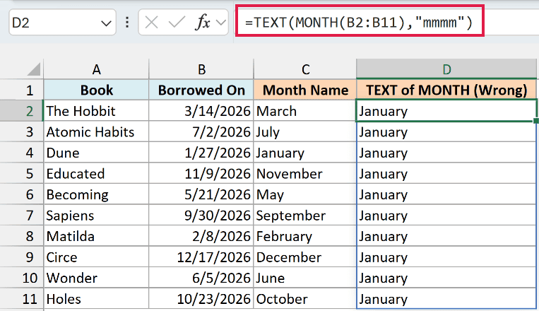
Every row in column D says January, even though the books were borrowed in all different months.
This happens because MONTH hands the TEXT function a plain number like 3, not a date. It reads 3 as a date serial number, which is January 3, 1900, so the month always comes out as January.
Example 3: Fix MONTH Returning 1 for Blank Cells
This next one gives a wrong answer without any warning.
Below is a list of job applicants with their interview dates, where some dates haven’t been set yet, and I want the interview month in column C.
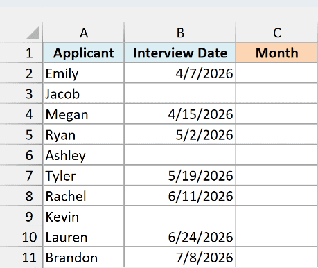
Here is the formula:
=MONTH(B2:B11)
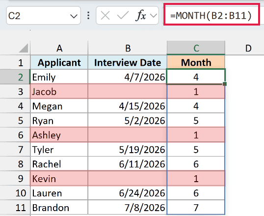
Look at Jacob, Ashley, and Kevin. Their interview dates are blank, but MONTH still gives each of them a 1, which looks exactly like a real January date.
Excel treats an empty cell as 0, and 0 as a date is January 0, 1900. So MONTH reads the blank as a January date and returns 1.
To leave those rows empty, check for a blank first. Here is the formula for column D:
=IF(B2:B11="","",MONTH(B2:B11))
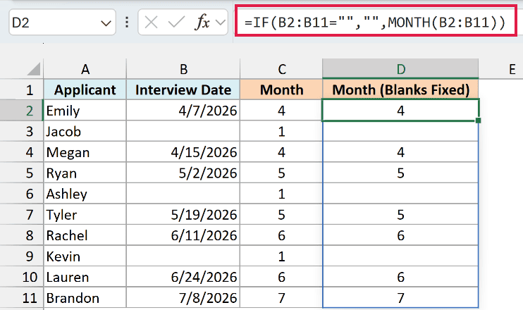
The IF function checks each date. When the cell is blank, it returns an empty text string (“”), and when there’s a date, it returns the month number.
Those blank-looking cells in column D hold text, not numbers. So a calculation that points at one of them, like =D3+1, returns a #VALUE! error.
Important: If you later count or average these month numbers, the plain MONTH version would add a fake January for every blank date. Use the IF version whenever your date column can have gaps.
Example 4: Convert a Month Name to a Number
Now let’s go the other way.
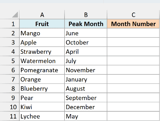
Below is a list of fruits with the month each one is in peak season, written as a name, and I want the month number in column C.
Here is the formula:
=MONTH(B2:B11&1)
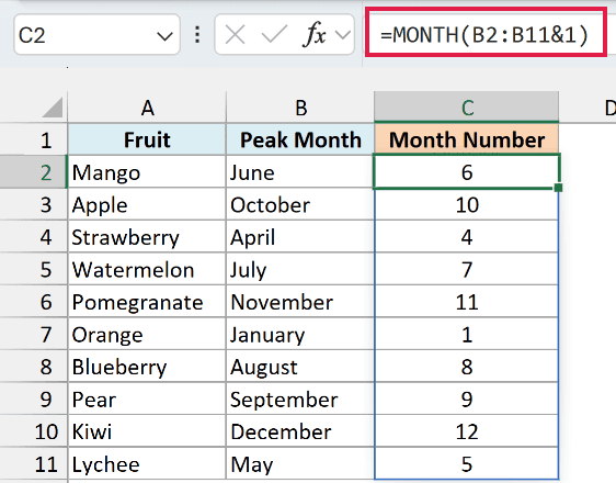
MONTH needs a date, and “June” on its own isn’t one. Adding &1 joins a 1 to the end of each name, so “June” becomes “June1”, which Excel reads as the date June 1.
MONTH then pulls the month out of that date, so June gives 6 and December gives 12.
This trick works only when Excel recognizes the text as a month name. A misspelled name like “Febuary” gives a #VALUE! error, so it’s worth a quick check of the names first.
Example 5: Find the Quarter From a Date
Here’s another practical scenario.
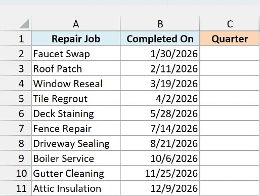
Below is a list of home repair jobs with the date each one was completed, and I want the quarter, like Q1, in column C.
Here is the formula:
="Q"&ROUNDUP(MONTH(B2:B11)/3,0)
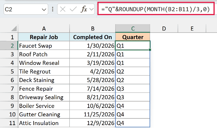
How this formula works:
- MONTH(B2:B11) gets the month number for each date, from 1 to 12.
- /3 divides that by 3, because every quarter has three months. So April (4) becomes 1.33 and December (12) becomes 4.
- ROUNDUP(…,0) rounds each result up to the next whole number, so 1.33 becomes 2. Months 1 to 3 end up as 1, months 4 to 6 as 2, and so on.
- “Q”& puts the letter Q in front, so 2 shows as Q2.
Example 6: Calculate the Fiscal Year for a Date
Let’s step it up a little.
Below is a list of office supply orders with their order dates, and I want the fiscal year for each order in column C, where the fiscal year starts on April 1.
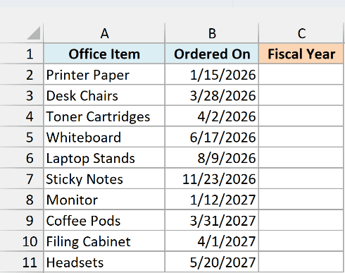
Here is the formula:
=YEAR(B2:B11)+(MONTH(B2:B11)>=4)
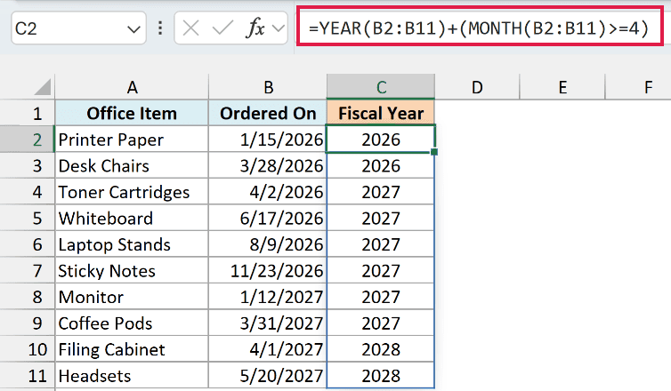
How this formula works:
- YEAR(B2:B11) gets the calendar year of each date.
- (MONTH(B2:B11)>=4) checks whether the month is April or later, and returns TRUE or FALSE for each date.
- When you add TRUE to a number, Excel counts it as 1, and FALSE counts as 0. So dates from April onward get one year added, and dates from January to March keep their calendar year.
This names each fiscal year after the calendar year it ends in. So April 2026 to March 2027 is fiscal year 2027.
You can see the switch at the bottom of the list. The Coffee Pods order on 3/31/2027 is still fiscal 2027, while the Filing Cabinet order the very next day, 4/1/2027, moves to 2028.
If your fiscal year starts in a different month, change the 4 to that month’s number, such as 7 for July.
Example 7: Get the First Day of the Month
This time the result is a full date, not a number.
Below is a list of customer orders with their order dates, and I want the first day of each order’s month in column C.
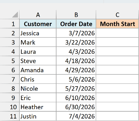
Here is the formula:
=DATE(YEAR(B2:B11),MONTH(B2:B11),1)
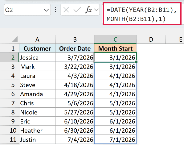
The DATE function builds a date from a year, a month, and a day. Here, the YEAR and MONTH functions take the year and month from each order date, and the day is fixed at 1.
So Jessica’s order on 3/7/2026 and Mark’s order on 3/22/2026 both become 3/1/2026. Every order from the same month now shares one date, which makes it easy to group them in a pivot table or count them with the COUNTIF function.
Unlike a plain month number, this keeps the year, so March 2026 and March 2027 never get mixed up.
If the results show up as numbers like 46082 instead of dates, the cells just need a date format. Select them and pick Short Date from the Number Format drop-down on the Home tab.
Example 8: Sum and Count Values by Month
Let’s finish with something a bit more advanced.
Below is a list of client payments with the date and amount of each one, and I want the total received and the number of payments for the month number I type in F1.
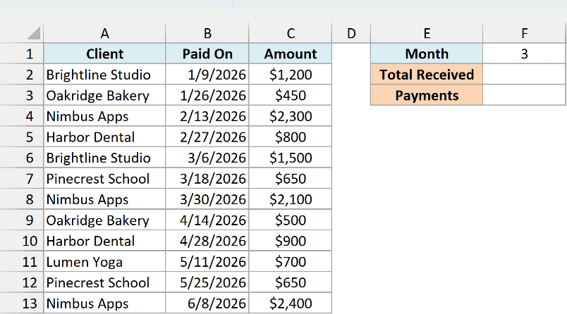
Here is the formula for the total in F2:
=SUM((MONTH(B2:B13)=F1)*C2:C13)
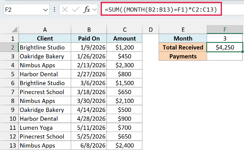
With 3 in F1, this returns $4,250, which is the three March payments added together (1,500 + 650 + 2,100).
How this formula works:
- MONTH(B2:B13)=F1 checks the month of every payment date against F1 and returns TRUE for the March dates and FALSE for the rest.
- C2:C13 holds the amounts, and the multiplication sign multiplies them by those TRUE and FALSE values. TRUE counts as 1 and FALSE as 0, so only the March amounts survive and every other amount becomes 0.
- SUM adds up what’s left.
Here is the formula for the count in F3:
=SUM(--(MONTH(B2:B13)=F1))
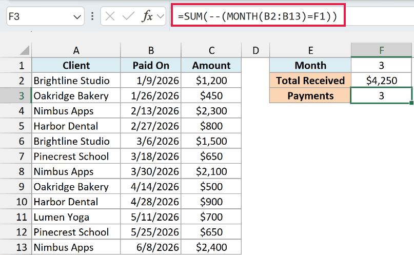
This returns 3. The two minus signs (–) turn each TRUE into 1 and each FALSE into 0, so SUM ends up counting the March dates.
Change F1 to 5, and both cells update to show the May numbers instead.
You might wonder why I’m not using the SUMIF or COUNTIF function here. Those functions need a range of cells to check, and MONTH(B2:B13) is a calculated list, so Excel won’t accept it there.
Important: These formulas check the month only, not the year. If your data covers more than one year, March 2025 and March 2026 both get counted, so add a year check too, like (YEAR(B2:B13)=2026).
The SUM versions above rely on newer Excel handling the list of TRUE and FALSE values, so older versions need Ctrl + Shift + Enter for them. The SUMPRODUCT function handles the list on its own and works with a normal Enter.
If you are using Excel 2019 or earlier, enter the below formula in cell F2 for the total:
=SUMPRODUCT((MONTH(B2:B13)=F1)*C2:C13)
And enter the below formula in cell F3 for the count:
=SUMPRODUCT(--(MONTH(B2:B13)=F1))
So that’s how the MONTH function works. On its own it just returns a number from 1 to 12, but paired with functions like TEXT, DATE, YEAR, or SUM, it handles month names, quarters, fiscal years, and monthly totals.
I hope you found this article helpful.
Other Excel Articles You May Also Like:
