EDATE Function in Excel

If you want to move a date forward or backward by a set number of months, the EDATE function in Excel gives you the new date.

It counts calendar months, so one month after 1/31/2026 is 2/28/2026.

In Excel 365, EDATE can take a column of dates and spill results below, with a plus-sign trick I’ll explain first.

In this article, I’ll show you how to use EDATE with eight practical examples, including adding years and keeping the time on a date.

Excel EDATE Function Syntax

Here is the syntax of the EDATE function:

=EDATE(start_date, months)

• start_date is the date you want to start from. Use a cell holding a real Excel date, a date serial number, or a formula that returns a date.
• months is the number of months to shift. Use a positive number to go forward, a negative number to go back, and 0 to return the same date.

Both arguments are required. EDATE returns a serial number, which is how Excel stores a date. Format the result cell as a date to see it that way.

The function keeps the same day number when it exists in the target month. If it doesn’t, EDATE returns the last day of that month.

If you enter a decimal for months, EDATE drops the decimal part rather than rounding it.

If you type a date in quotes inside the formula, Excel reads it using your regional date settings.

For example, =EDATE("1/31/2026",1) may work on one machine and return #VALUE! on another with different regional date settings.

Important: To avoid this problem, use a cell holding a real date, or build it with the DATE function.

EDATE is available in Excel 365, 2024, 2021, 2019, and 2016, as well as Excel for Mac and Excel on the web.

When to Use the EDATE Function

Use this function when you need to:

• Shift dates by whole calendar months instead of treating every month as 30 days.
• Calculate renewal dates, deadlines, or maturity dates from a start date.
• Apply a different month count to each row in a list.
• Generate monthly or quarterly dates from one starting date.
• Set moving date windows for filters and alerts.

If you always want the last day of the target month, use the EOMONTH function instead. I’ll show you the difference in the final example.

Let me show you a few practical examples of how this works.

Example 1: Add Months to a Whole Column

Let’s start with how to add months to a date for a whole column at once.

Below I have gym members’ last renewal dates, and I want to calculate their next quarterly renewal, three months later, in column C.

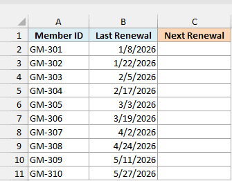
Here is the formula:

=EDATE(+B2:B11,3)

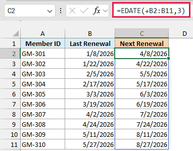
In Excel 365, this single formula spills the ten renewal dates into C2:C11. You type it once in C2 and Excel fills the rest.

The 3 tells EDATE to move each date forward three months. GM-301’s 1/8/2026 becomes 4/8/2026, and GM-310’s 5/27/2026 becomes 8/27/2026.

Important: =EDATE(B2:B11,3) returns #VALUE!. The plus in +B2:B11 turns the range reference into an array of values that EDATE can use.

EDATE was originally an Analysis ToolPak add-in function. It still doesn’t accept a bare range reference as an array, which is why that plus sign matters.

The guide to Excel functions that won’t spill explains this behavior in more detail.

In Excel 2019 and earlier, enter =EDATE(B2,3) in C2 and copy it down to C11 instead.

After entering the formula, you may see 46120 in C2 instead of 4/8/2026. That’s Excel’s date serial number, so the result is right.

Select the result cells and apply a Date format to display the dates.

If you get #SPILL! instead of dates, check that the cells below C2 are empty so Excel has room for the results.

A spilling formula also can’t sit inside an Excel Table, so place it outside the table.

Example 2: Subtract Months From a Date

Now let’s go the other way and shift dates backward instead of forward.

Below is an exam schedule, and I want to find the registration deadline two months before each exam in column C.

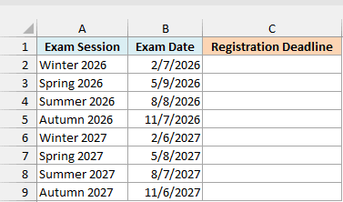
Here is the formula:

=EDATE(+B2:B9,-2)

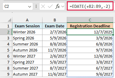
The only change from the first example is the negative 2. That tells EDATE to move backward two months. The deadlines spill into C2:C9.

Winter 2026 has an exam date of 2/7/2026 and a registration deadline of 12/7/2025. EDATE handles the year change without an extra calculation.

For Spring 2026, the exam on 5/9/2026 gets a deadline of 3/9/2026. The day number stays the same.

Example 3: Use Different Months Per Row

The number of months doesn’t have to be the same for every row, so let’s use a separate column of month counts.

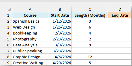
Below I have online courses with their start dates and lengths in months, and I want to calculate each course’s end date in column D.

Here is the formula:

=EDATE(+B2:B9,+C2:C9)

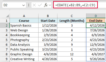
Here, the months argument is a range instead of a single number. Excel pairs each start date in B2:B9 with the length on the same row in C2:C9.

Spanish Basics starts on 1/12/2026 and runs for 3 months, giving 4/12/2026. Web Design starts on 1/26/2026 and runs for 6 months, giving 7/26/2026.

Both bare ranges need a plus sign. Leaving it off the months range, as in =EDATE(+B2:B9,C2:C9), gives #VALUE! in the first result.

With both plus signs in place, the eight end dates spill into D2:D9.

Example 4: Generate Quarterly Due Dates

Sometimes you don’t have a column of dates at all, just one starting date and a series of payments to schedule.

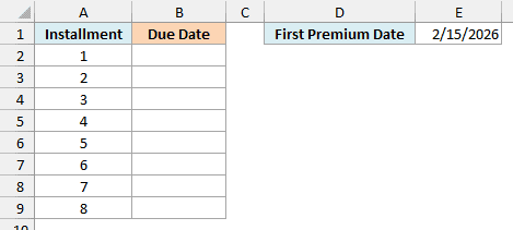
Below is a car insurance premium schedule, and I want eight quarterly due dates, starting with the first premium date, in column B.

E1 holds the first premium date, 2/15/2026.

Here is the formula:

=EDATE(E1,SEQUENCE(8,,0,3))

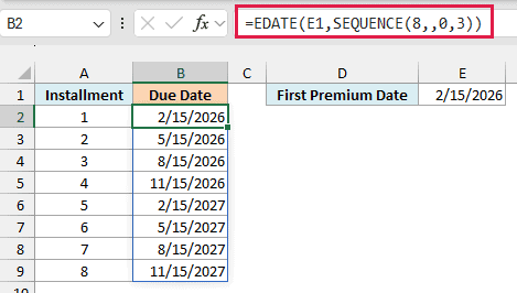
The dates spill into B2:B9, starting at 2/15/2026 and ending at 11/15/2027.

Here is how this formula works:

• SEQUENCE(8,,0,3) generates eight month offsets: 0, 3, 6, 9, 12, 15, 18, and 21. The blank second argument gives a single column.
• EDATE shifts the date in E1 by each offset. The 0 keeps the first date, and each later offset moves it forward another three months.
• E1 is a single cell and SEQUENCE already returns an array, so neither argument needs a plus sign.

The 8 controls how many dates you get. Change it to 12 for three years of quarterly dates, or change the 3 to 1 for monthly dates.

The SEQUENCE function needs Excel 365 or Excel 2021 and later.

Example 5: Add Years to Dates With EDATE

You can also add years to a date with EDATE by converting the years to months.

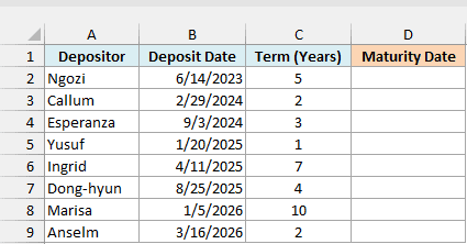
Below I have fixed deposits with their deposit dates and terms in years, and I want to calculate each maturity date in column D.

Here is the formula:

=EDATE(+B2:B9,C2:C9*12)

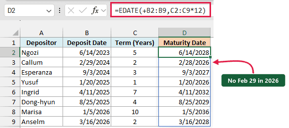
The maturity dates spill into D2:D9.

Here is how this formula works:

• +B2:B9 gives EDATE the deposit dates as an array of values.
• C2:C9*12 multiplies each term by 12 to convert years into months. One year becomes 12 months, so this also covers adding 12 months to a date.
• EDATE shifts each deposit date by its own month count. The multiplication already turns C2:C9 into an array, so that argument needs no plus sign.

Ngozi’s 5-year deposit on 6/14/2023 matures on 6/14/2028. Yusuf’s 1-year deposit on 1/20/2025 matures on 1/20/2026.

Callum’s deposit starts on 2/29/2024 and has a 2-year term. The maturity date is 2/28/2026 because 2026 has no February 29.

Example 6: List Reviews Due Within Three Months

Now let’s use EDATE to set the end of a date window and pull out only the reviews that fall inside it.

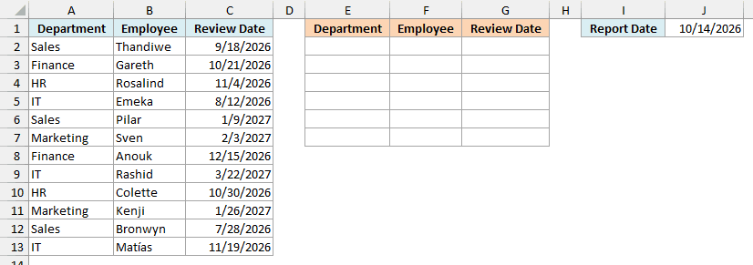
Below is a list of employee performance reviews, and I want those due from the report date through three months later, including both dates, in columns E to G.

J1 holds the report date, 10/14/2026.

Here is the formula:

=FILTER(A2:C13,(C2:C13>=J1)*(C2:C13<=EDATE(J1,3)),"None due")

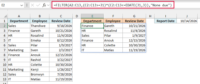
The six matching reviews spill into E2:G7 in source order: Gareth, Rosalind, Pilar, Anouk, Colette, and Matías.

Here is how this formula works:

• EDATE(J1,3) returns 1/14/2027, which is the end of the three-month window.
• C2:C13>=J1 checks whether each review is on or after 10/14/2026.
• C2:C13<=EDATE(J1,3) checks whether each review is on or before 1/14/2027.
• Multiplying the conditions converts TRUE/FALSE into 1/0. A row gives 1 only when both conditions are TRUE, so FILTER keeps only those rows.
• "None due" is the message FILTER returns when nothing matches, instead of a #CALC! error.

Pilar’s review on 1/9/2027 is included. Kenji’s 1/26/2027 review is just past the window, and Thandiwe’s 9/18/2026 review is before it.

The FILTER function needs Excel 365 or Excel 2021 and later.

Pro Tip: Use TODAY() instead of J1 for daily updates: =FILTER(A2:C13,(C2:C13>=TODAY())*(C2:C13<=EDATE(TODAY(),3)),"None due").

The example file uses a fixed report date so its results match the screenshots. With the TODAY function, the window moves as the date changes.

Example 7: Shift Dates and Keep the Time

If your cells hold a date and a time together, EDATE returns the shifted date at midnight, so let’s put the original time back.

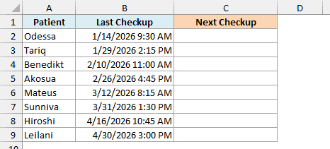
Below I have dental checkup dates and times, and I want to schedule each next checkup six months later at the same time in column C.

Columns B and C use m/d/yyyy h:mm AM/PM to display both the date and the time.

Here is the formula:

=EDATE(+B2:B9,6)+MOD(B2:B9,1)

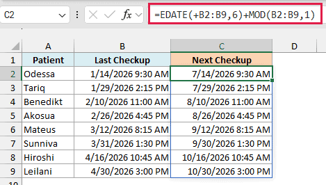
The next checkup dates and times spill into C2:C9. Odessa’s 1/14/2026 9:30 AM becomes 7/14/2026 9:30 AM.

Here is how this formula works:

• EDATE(+B2:B9,6) shifts each date forward six months but drops the time, returning midnight.
• Excel stores the time of day as the decimal part of a date’s serial number. MOD(B2:B9,1) returns that decimal for each appointment.
• Adding the two parts restores the original time on the shifted date. MOD accepts the range directly, so it needs no plus sign.

Sunniva’s 3/31/2026 1:30 PM becomes 9/30/2026 1:30 PM. September has 30 days, so EDATE uses the last day and MOD keeps the 1:30 PM time.

A Date-only format hides the time even when the formula has kept it. Make sure that the result cells use a date-and-time number format.

You can read more about extracting remainders in the MOD function tutorial.

Example 8: EDATE vs EOMONTH at Month-End

Let’s finish by comparing what EDATE and EOMONTH return when signup dates fall at or near the end of a month.

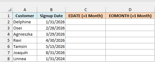
Below is a list of subscription signup dates, and I want to compare the EDATE and EOMONTH results for one month later in columns C and D.

Here is the formula:

=EDATE(+B2:B8,1)

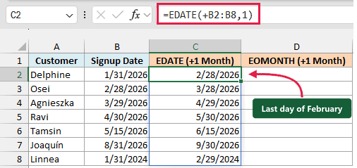
The dates spill into C2:C8. EDATE keeps the day number where it can: Agnieszka’s 3/29/2026 becomes 4/29/2026, and Tamsin’s 5/15/2026 becomes 6/15/2026.

Delphine’s 1/31/2026 becomes 2/28/2026, and Joaquín’s 8/31/2026 becomes 9/30/2026. Those target months have no 31st, so EDATE uses their last day.

Now let’s calculate the last day of the following month for each signup by entering the EOMONTH formula in D2.

Here is the formula:

=EOMONTH(+B2:B8,1)

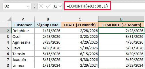
These dates spill into D2:D8. Agnieszka’s result is now 4/30/2026, and Tamsin’s is 6/30/2026, because EOMONTH always returns month-end.

The difference is that EDATE keeps the original day number unless it doesn’t exist in the target month. EOMONTH always returns the target month’s last day.

In this dataset, the formulas agree only where EDATE has to use the month’s last day: Delphine, Joaquín, and Linnea.

Linnea’s 1/31/2024 becomes 2/29/2024 with both functions. That row shows how they handle February in a leap year.

Pro Tip: Osei’s month-end date, 2/28/2026, becomes 3/28/2026 with EDATE, not 3/31/2026. If your rule is “always the last day of the month,” use the EOMONTH function.

I’ve shown you how to shift dates by months or years, build a date window, and keep the time when you need it.

EDATE doesn’t count weeks. To add weeks to a date, add 7 times the number of weeks to the date.

For working days that skip weekends and holidays, use the WORKDAY function.

I hope you found this article helpful.

List of All Excel Functions

Other Excel Articles You May Also Like:

• How to Add or Subtract Days to a Date in Excel
• Calculate Number of Months Between Two Dates in Excel
• DATEDIF Function in Excel
• DAY Function in Excel (5 Examples)
• How to Get the Number of Days in a Month in Excel?
• How to Get the First Day of the Month in Excel (Easy Formulas)
• Calculate Fiscal Year from Date in Excel (Formulas)
• How to Calculate Years of Service in Excel (Easy Formulas)